
B
ACKGROUND SUBTRACTION WITH ADAPTIVE
SPATIO-TEMPORAL NEIGHBORHOOD ANALYSIS
Marco Cristani and Vittorio Murino
Computer Science Dep., Universit
`
a degli Studi of Verona, Strada Le Grazie 15, Verona, Italy
Keywords:
Surveillance, Motion analysis, Robustness.
Abstract:
In the literature, visual surveillance methods based on joint pixel and region analysis for background sub-
traction are proven to be effective in discovering foreground objects in cluttered scenes. Typically, per-pixel
foreground detection is contextualized in a local neighborhood region in order to limit false alarms. However,
such methods have an heavy computational cost, depending on the size of the surrounding region considered
for each pixel. In this paper, we propose an original and efficient joint pixel-region analysis technique able
to automatically select the sampling rate with which pixels in different areas are checked out, while adapting
the size of the neighborhood region considered. The algorithm has been validated on standard videos with
benchmark tests, proving the goodness of the approach, especially in terms of quality of the detection with
respect to the frame rate achieved.
1 INTRODUCTION
Background subtraction is a fundamental step in auto-
mated video surveillance. It aims at classifying pixel
values as background (BG), i.e., the expected part of
the monitored scene, and the foreground (FG), i.e., the
interesting visual information (e.g., moving objects).
It is widely accepted that BG subtraction cannot be
adequately performed by per-pixel methods, i.e., con-
sidering every temporal pixel evolution as an indepen-
dent process. Instead, per-pixel methods augmented
with per-region strategies (also called hybrid meth-
ods, see Section 2) better behave, deciding the class
of a pixel value by inspecting the related neighbor-
hood. Using hybrid schemes, several BG subtraction
issues can be effectively faced (Toyama et al., 1999);
anyway, the price to pay in hybrid systems is undoubt-
edly an increase of the computational load required.
In this paper, we propose a hybrid BG subtrac-
tion scheme which gives two contributes to the related
state of the art: first, it is accurate, i.e., the number
of false alarms is low: this is due to a dynamic def-
inition of the neighborhood zone around each pixel
which permits to capture aperiodic chromatic oscil-
lations of scene components, such as boats in a har-
bour scenario or moving tree branches. Second, our
method is fast, outperforming the time performances
of the most-known BG subtraction algorithms. In
practice, zones where the background is static with
the same visual aspect are seldom observed. Vice
versa, zones where the background varies or where
foreground is visible are examined more often. We
call our method adaptive spatio-temporal neighbor-
hood analysis (ASTNA). Experiments carried out on
standard and ad-hoc benchmark data show the good-
ness of ASTNA.
The rest of the paper is organized as follows. Sec-
tion 2 reviews briefly the state of the art of the back-
ground subtraction methods; details of the proposed
strategy are reported in Section 3; in Section 4, ex-
periments on real data and critical observations are
reported, and, finally, in Section 5 conclusions are
drawn and future perspectives envisaged.
2 RELATED LITERATURE
The actual BG subtraction literature is large and mul-
tifaceted; here we propose a taxonomy in which the
BG subtraction methods are organized in i) per pixel,
ii) per region, iii) per frame, and iv) hybrid methods.
The class of per-pixel approaches is formed by meth-
ods that perform BG/FG discrimination by consider-
ing each pixel signal as an independent process. One
of the first BG modeling was proposed in the surveil-
lance system Pfinder (Wren, et al., 1997), where
each pixel signal was modeled as a uni-modal Gaus-
sian distribution. In (Stauffer and Grimson, 1999),
484
Cristani M. and Murino V. (2008).
BACKGROUND SUBTRACTION WITH ADAPTIVE SPATIO-TEMPORAL NEIGHBORHOOD ANALYSIS.
In Proceedings of the Third International Conference on Computer Vision Theory and Applications, pages 484-489
DOI: 10.5220/0001072704840489
Copyright
c
SciTePress

the pixel evolution is modeled as a multimodal sig-
nal, described with a time-adaptive mixture of Gaus-
sian components (TAPPMOG). In (Suter and Wang,
2005), the authors specified i) how to cope with color
signals (the original version was proposed for gray
values), proposing a normalization of the RGB space
taken from (Mittal and Paragios, 2004), ii) how to
avoid overfitting and underfitting (due to values of the
variances too low or too high), proposing a thresh-
olding operation, and iii) how to deal with sudden
and global changes of the illumination, by tuning the
learning rate parameter. For the latter, the idea was
to increase the learning rate when the foreground in-
creases from one frame to another more than 70%: in
this way the BG model can faster evolve and produce
less false alarms. Note that this model cannot more
be called TAPPMOG, because global reasoning is ap-
plied.
In (Zivkovic, 2004), the number of Gaussian com-
ponents is automatically chosen, using a Maximum
A-Posteriori (MAP) test and employing a negative
Dirichlet prior, able to associate more than a single
Gaussian component where the BG exhibits a mul-
timodal behavior, thus allowing a faster BG mainte-
nance.
Another per-pixel approach is proposed in (Mittal and
Paragios, 2004): this model uses a non-parametric
prediction algorithm to estimate the probability den-
sity function of each pixel, which is continuously up-
dated to capture fast gray level variations. In (Nakai,
1995), pixel value probability densities, represented
as normalized histograms, are accumulated over time,
and BG label are assigned by the Maximum A Poste-
riori criterion.
Region-based algorithms usually divide the frames
into blocks and calculate block-specific features;
change detection is then achieved via block match-
ing, considering for example fusion of edge and in-
tensity information (Noriega and Bernier, 2006). In
(Heikkila and Pietikainen, 2006) a region model de-
scribing local texture characteristic is presented:the
method is prone to errors when shadows and sudden
global changes of illumination occur.
Frame-level class is formed by methods that look for
global changes in the scene. Usually, they are used
jointly with other pixel or region BG subtraction ap-
proaches. In (Stenger et al., 2001), a graphical model
was used to adequately model illumination changes of
the scene. In (Ohta, 2001), a BG model was chosen
from a set of pre-computed ones, in order to minimize
massive false alarm.
Hybrid models describe the BG evolution using
jointly pixel and region models, and adding in gen-
eral post-processing steps. In Wallflower (Toyama et
al., 1999), a 3-stage algorithm is presented, which op-
erates respectively at pixel, region and frame level.
Wallflower test sequences are widely used as compar-
ative benchmark for BG subtraction algorithms. In
(Wang and Suter, 2006), a non parametric, per pixel
FG estimation is followed by a set of morphological
operations in order to solve a set of BG subtraction
common issues. In (Kottow et al., 2004) a region level
step, in which the scene is modeled by a set of local
spatial-range codebook vectors, is followed by an al-
gorithm that decides at the frame-level whether an ob-
ject has been detected, and several mechanisms that
update the background and foreground set of code-
book vectors. For a good BG subtraction methods re-
view, see (Piccardi, 2004).
3 PROPOSED METHOD
Let n, n = 1,... ,N be a pixel location, z
n
be the pixel
signal observed at location n and z
(t)
n
be a realization
of such signal at time t. The decision to classify z
(t)
n
as BG or FG is given by a two-step process. The first
step is the per-pixel (PP) process, the second step is
the per-region (PR) process.
3.1 The Per-pixel Process
The PP process controls whether the per-pixel infor-
mation is sufficient to explain z
(t)
n
as a BG value. In
this paper, each pixel signal is modeled using a set
of R Gaussian pdf’s N (·), as proposed by (Stauffer
and Grimson, 1999). The probability of observing the
value z
(t)
n
is:
P(z
(t)
n
) =
R
∑
r=1
w
(t)
n,r
N (z
(t)
n
|µ
(t)
n,r
,σ
(t)
n,r
) (1)
where w
(t)
n,r
, µ
(t)
n,r
and σ
(t)
n,r
are the time adaptive mix-
ing coefficients, the mean, and the standard deviation,
respectively, of the r-th Gaussian of the mixture as-
sociated with z
(t)
n
. At each time instant, the Gaus-
sian components are evaluated in descending order
with respect to w/σ to find the first matching with
z
(t)
n
(a match occurs if the value falls within 2.5σ of
the mean of the component). If no match occurs, the
least ranked component is replaced with a new Gaus-
sian with the mean equal to the current value, high
variance and a low mixing coefficient. If r
hit
is the
matched Gaussian component, the value z
(t)
is labeled
FG if
r
hit
∑
r=1
w
(t)
r
> T (2)
BACKGROUND SUBTRACTION WITH ADAPTIVE SPATIO-TEMPORAL NEIGHBORHOOD ANALYSIS
485

where T is a standard threshold, the summation
∑
r
hit
r=1
w
(t)
r
represents the probability that the Gaussian
components considered do model the background.
We call the test in (2) as the background per-pixel test
(BG PP test), which is true (= 1) if the value is labeled
BG (z
(t)
n
∈BG), false (= 0) vice versa. For further de-
tails, see (Stauffer and Grimson, 1999).
3.2 The Per-region Process
If z
(t)
n
is not recognized as BG by the BG PP test, then
the PR process determines if z
(t)
n
is similar to another
BG signal value, located in a close position n
0
. In
formulae, z
(t)
n
is labeled BG by the PR process if the
following background per-region test (BG PR test) is
true:
_
n
0
∈G
n
³
z
(t)
n
∈ N (µ
n
0
,
˜
k
,σ
n
0
,
˜
k
)
^
z
(t)
n
0
∈ BG
´
(3)
where
W
,
V
indicate or and and operators respec-
tively, G
n
is the squared neighborhood zone related to
location n and
˜
k addresses whatever Gaussian compo-
nent that models the pixel location n
0
, which satisfies
the condition above. Eq.(3) is true if z
(t)
n
matches with
a particular Gaussian component located at position
n
0
and the signal value z
(t)
n
0
, modeled by such Gaus-
sian pdf, is labeled BG by the PP process. The BG
labeling mechanism exploited in the PR process mir-
rors the policy proposed in (Elgammal et al., 2000). If
some part of the background (a tree branch for exam-
ple) moves to occupy a new pixel, but it was not part
of the per-pixel model for that pixel, then it will be de-
tected as a FG object by a classical per-pixel method.
However, this object will have a high probability to
be a part of the BG distribution in its original posi-
tion. Clearly, the bigger the neighborhood zone G
n
,
the heavier will be the computational load required
for evaluating Eq.(3). In this paper, we propose to
adopt a strategy for changing G
n
on-line, in order to
turn down the computational effort. From here, we
indicate with s
(t)
n
half the size of the neighborhood
zone G
n
at time t, resulting in a square of odd size
1 + 2s
(t)
n
. At time t = 0, s
(0)
n
= s
min
, where s
min
in-
dicates the smallest length permitted. In this paper,
we set s
min
as 0, resulting in a neighborhood zone of
a single pixel location. At time t = 1, if the BG PP
test is negative (i.e., we have a FG per-pixel detection
at location n), the PR process does not contributes to
find a BG neighborhood signal similar to z
(1)
n
; there-
fore, the whole process will give a FG detection at
position n. After this, s
n
is enlarged by a factor γ
s
,
obtaining a squared region of size b1 + 2 ∗ γ
s
c. If the
PR+PP process continues to identify a FG value at po-
sition n, a maximal length s
max
is considered. Vicev-
ersa, if the PR test is positive, we have a BG detection,
and the growing process of s
n
stops. Conversely, let
us suppose that at frame t the BG PP test is positive.
This means that the per-pixel statistic is enough to ex-
plain the pixel signal z
(t)
n
as a BG instance. Therefore,
having a large neighborhood zone of size s
n
to ana-
lyze brings to a useless computational burden. Con-
sequently, the size s
(t)
n
is diminished by the factor γ
s
.
Hence, if the PP BG test continues to be positive, then
s
n
is diminished until the smallest size s
min
is reached.
Summarizing, the size of s
(t)
n
changes as follows:
s
(t)
n
=
s
max
if PP test=0∧
PR test=0 ∧ s
(t−1)
n
=s
max
s
(t−1)
n
+ γ
s
if PP test=0 ∧ PR test=0
s
(t−1)
n
if PP test=0 ∧ PR test=1
s
(t−1)
n
− γ
s
if PP test=1 ∧ s
(t−1)
n
>s
min
s
min
if PP test=1 ∧ s
(t−1)
n
=s
min
(4)
A graphical example of the process is given in Fig.1.
When the smallest size s
min
has been reached for
the location n, if the signal z
(t)
n
is detected as BG sim-
ply by the BG PP process, we decide to sample it ev-
ery bI(n)
(t)
c frames, where I(n)
(t)
is a skipping time
set initially to 0, which increments by a factor γ
t
each
time z
(t)
n
is discovered consecutively as BG by the BG
PP test. This happens until the maximal skip interval
I
max
is reached. During the skip, the Gaussian param-
eters that describe the signal z
n
are left unchanged.
This temporal sampling process stops immediately as
soon as the BG PP test is negative, and I(n)
(t)
is set to
0.
The quality of the results obtained justifies the
heuristic aspect of the proposed method.
4 EXPERIMENTS AND
DISCUSSION
Several tests have been performed to validate the pro-
posed approach. In the first benchmark, the well-
known “Wallflower” dataset (Toyama et al., 1999) has
been considered; it contains sequences which present
different hard BG subtraction issues; each sequence
has a ground truth frame. Here, we processed four
of the most difficult sequences of the dataset, i.e.,
sequences whose best BG subtraction results are far
from the ground truth. The sequences are: 1)Waving
Tree (WT): a tree is swaying and a person walks in
front of the tree; 2)Camouflage (C): a person walks in
front of a monitor, which has rolling interference bars
VISAPP 2008 - International Conference on Computer Vision Theory and Applications
486
z
n’
(1)
t=1
z
n
(2)
t=2,
BG PP test
t=2,
BG PR test
t=3,
BG PP test
t=3,
BG PR test
G
n
(2)
t=4,
BG PP test
+ BG PR test
z
m
(3)
z
l
(2)
G
m
(3)
G
n’
(1)
z
l
(3)
G
l
(3)
G
l
(4)
z
m
(2)
z
n’
(2)
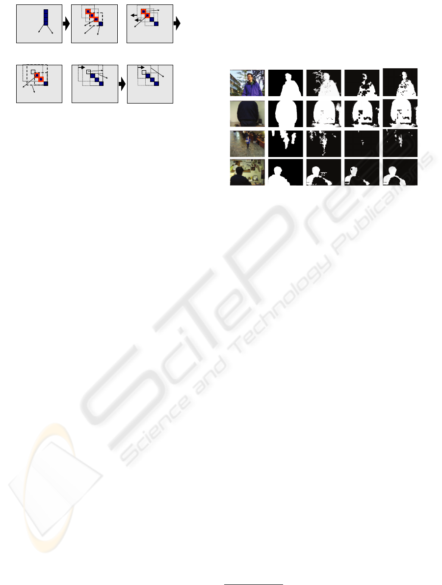
Figure 1: Scheme of ASTNA: At time t = 1, suppose that
only the blue pixels are sampled. At time t = 2 location z
(2)
n
is detected as FG (the pixel is rounded by a red square) by
the BG PP test, but the BG PR test is positive, having the
region G
(2)
n
a BG pixel value z
0(2)
n
similar to z
(2)
n
inside. The
other values z
(2)
l
and z
(2)
m
are detected as FG by the PR BG
test, thus their neighborhood zones are enlarged. At time
t = 3 the value z
(3)
m
is labelled BG by the PR test, while
the pixel value z
(3)
l
is labelled BG by the PP test, and its
neighborhood zone can be diminished. Only BG values are
detected at time t = 4.
on the screen. The bars include color similar to the
persons clothing; 3)Bootstrapping (B): a busy cafe-
teria where each frame contains FG objects; 4)Fore-
ground Aperture (FA): a person with uniformly col-
ored shirt wakes up and begins to move. Consider-
ing the other three Wallflower sequences, two of them
refer i) to the capacity of the background model to
incorporate a moved object in the background model
after a reasonable time it is still, and ii) to the capacity
of the background model to adapt to a gradual change
of illumination. Both these problems are solved by
the ordinary TAPPMOG, and thus our model does not
add any deterioration in the performance. The third
sequence present an instance of the sudden global
change in illumination issue. Our method fails in this
case, being absent a per-frame module. Anyway, such
problem does not represent an important issue, be-
ing present several techniques able to solve it with
very low computational effort (for example, using a
set of pre-learnt global model of the scene, and using
the most appropriate, as done in (Ohta, 2001)). An-
other issue that we do not face in this papers are the
shadows issue, another problem in video surveillance.
This will be addressed in a future work, as explained
in the last section.
All the RGB sequences are captured at resolution
of 160 × 120 pixels, sampled at 4Hz. In our pure
MATLAB implementation, on a Pentium IV, 3Ghz,
1Gb RAM, we set A
max
= 5,I
max
= 4, γ
s
= γ
t
= 0.2;
such quantities are intuitive and easy to set. For each
sequence, we show qualitative results in Fig.2: for
lack of space only the results related to the TAPP-
MOG (Stauffer and Grimson, 1999) and Elgammal
(Elgammal et al., 2000) methods are reported
1
): for
a more extensive listing of the existent results, please
see (Toyama et al., 1999). In Fig.3, a wider set of
WT
C
B
FA
Figure 2: Wallflower qualitative results: on the 1st col.,
the test frames; on the 2nd col. the ground truth; the 3rd
col. shows the TAPPMOG results; Elgammal results and
results obtained with our method ASTNA are on the last
two columns, respectively.
quantitative results are provided in terms of amount
of false positive and false negative FG detections.
In particular, Wallflower, SACON, Tracey Lab LP
and Bayesian Decision refer to (Toyama et al., 1999;
Wang and Suter, 2006; Kottow et al., 2004; Nakai,
1995) respectively, which have been previously dis-
cussed in Section 2.
As visible, all the results provided by ASTNA
are comparable with the best performances obtained
by other techniques; in particular, our method reach
optimal results in the Waving Tree test, by correctly
modelling as BG the tree. In the Bootstrap test, our
method correctly considers as BG the light reflexes
on the floor, even if they are irregularly occurring
with sudden small displacements. This because our
method learns the zones of the scene in which oscil-
lating or flickering background is present, permitting
to use in those areas large neighborhood zones. At the
same time, zones in which the BG is still and stable
are considered as formed by independent pixel loca-
tions with minimal 1-pixel neighborhood zone, and,
as a consequence, they are more sensible to FG occur-
rences. Another observation is that our method can be
thought as improving the performances of the TAPP-
MOG method. Actually, TAPPMOG models over
the same pixel different Gaussian components, taking
into account different chromatic modes of the back-
ground. Our method permits to share these modes
among adjacent pixels locations, if necessary. One
1
Regarding the Elgammal method, the neighborhood
zone is represented by a fixed squared zone of size 5 for
all the pixel locations n = 1, ... ,N.
BACKGROUND SUBTRACTION WITH ADAPTIVE SPATIO-TEMPORAL NEIGHBORHOOD ANALYSIS
487
13019
3101
310
3411
2688
0
2688
823
1173
1996
2899
1
2900
f.neg.
f.pos.
t.e.
Elgammal
10059
2217
870
3087
1732
1033
2765
220
2398
2618
56
1533
1589
f.neg.
f.pos.
t.e.
TAPPMOG
14043
2501
1974
4485
2143
2764
4907
1538
2130
3688
629
334
963
f.neg.
f.pos.
t.e.
Bayesian
decision
7219
2403
356
2759
1974
92
2066
1998
69
2067
191
136
327
f.neg.
f.pos.
t.e.
Tracey LAB
LP
4084
1508
521
2029
1150
125
1275
47
462
509
41
230
271
f.neg.
f.pos.
t.e.
SACON
9170
320
649
969
2025
365
2390
229
2706
2935
877
1999
2876
f.neg.
f.pos.
t.e.
Wallflower
T.Err.FABCWTErr.
Methods
7031
1900
360
2260
2349
73
2422
2239
881
3120
253
100
353
f.neg.
f.pos.
t.e.
ASTNA
Figure 3: Quantitative results obtained by the proposed
ASTNA method: f.neg, f.pos.,t.e. and T.Err mean false
negative, false positive per-pixel FG detections, total er-
rors on the specific sequence and total errors summed on
all the sequences analyzed, respectively. Our method out-
performed the most effective general purposes BG subtrac-
tion scheme (Wallflower, Bayesian decision, TAPPMOG,
Elgammal), and is comparable with methods which are
more time demanding (see Tab.1) and strongly constrained
by data-driven initial hypotheses (SACON and Tracey Lab
LP).
Table 1: Times of execution in seconds of the different
BG subtraction methods when applied to the Wallflower se-
quences.
Methods WT C B FA
SACON 47.33 49.33 50.52 81.5
TAPPMOG 64.15 65.04 67.46 108.44
Elgammal 75.20 67.80 72.16 108.64
ASTNA 33.49 28.12 33.02 39.52
can afford that similar results can be provided by aug-
menting the number of per-pixel Gaussian compo-
nents, but doing this way occasional reflections of
the background cannot effectively be modeled. As
a further result, on Table 1 the total execution time
needed by the different algorithms to process the test
sequences is reported. One can notice the timings of
SACON, which is the only one that outperforms our
method for what concerns quality of the results. All
the other methods of Fig.3 not reported in Table 1 ex-
hibit worse performances.
These results show that ASTNA outperforms both
the fixed-neighborhood zones method (Elgammal et
al., 2000) and the classical TAPPMOG method. This
last result is due to the fact that the computational ef-
fort required by ASTNA to inspect a neighborhood
zone for each pixel is counterbalanced by the fact that
ASTNA avoids to sample locations with stable pixel
value at each iteration.
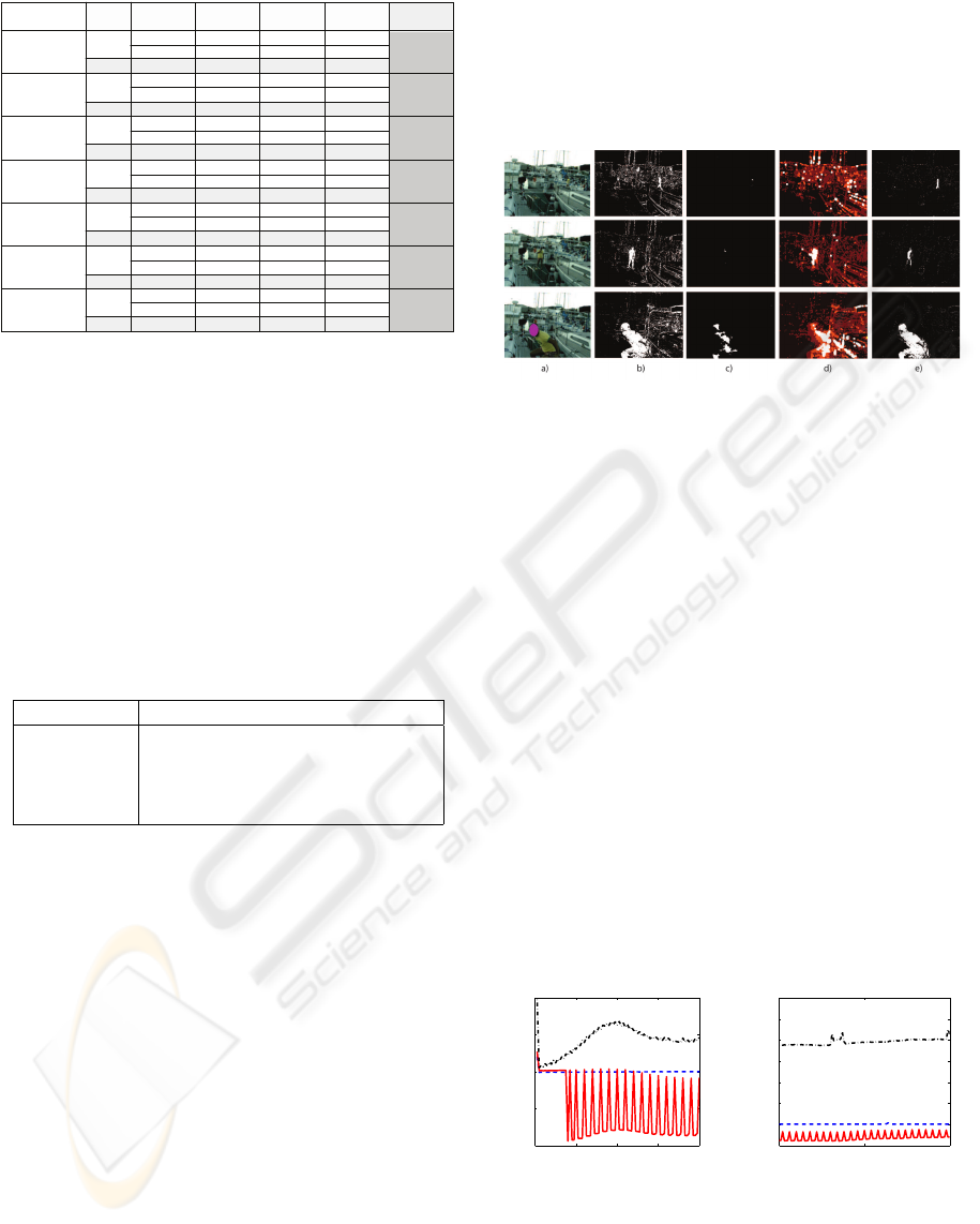
To give a better insight on how our method per-
forms, we consider another hard sequence, 320 × 240
pixels, 1170 frames long, in which a docking scenario
is portrayed. In Fig.4a) some frames are shown and
one can notice that reflecting sea and oscillating boats
are present.
Figure 4: Dock sequence: a) some frames of the sequence
(the face of the person is obscured due to the anonymity
issues); b) TAPPMOG results; c) Elgammal results; d)
ASTNA neighborhood image: brighter pixels mean wider
neighborhood zones for that pixel; d) ASTNA results. Note
that in all these results were not applied morphological op-
erations to clean up small FG detections.
During the sequence, a person arrives near the
camera, goes up on a boat, and lastly goes away. The
images in Fig.4d), at each pixel, indicate the area of
the related neighborhood zone calculated by our algo-
rithm. As one can note, our method considers bigger
zones only where significant oscillations are present
(near the masts). The time occurred for process such
sequence is 1478.20 sec. for Elgammal, 1067.60
sec. for TAPPMOG and 374.28 sec. for ASTNA.
In Fig.5, the time required for each iteration is re-
ported, for all the three methods, at different frames;
it is evident that our method is upper-bounded by the
fixed-neighborhood Elgammal technique, while out-
performs TAPPMOG method after the on-line learn-
ing of the most adapt neighborhood zones has been
performed.
0 20 40 60 80
0.8
0.85
0.9
0.95
1
frame
sec.
550 600 650
0
0.1
0.2
0.3
0.4
0.5
0.6
0.7
frame
sec.
Figure 5: Timings for the “Dock” sequence: the dashed
line, the point-dashed line and the solid line indicates TAPP-
MOG, Elgammal and ASTNA timings, respectively.
VISAPP 2008 - International Conference on Computer Vision Theory and Applications
488

5 CONCLUSIONS AND FUTURE
PERSPECTIVES
In this paper, we focus on producing a strategy which
is able to perform background subtraction in a fast and
robust way. The idea is to use an already present ef-
fective background subtraction technique, which op-
erates per-pixel, namely the TAPPMOG algorithm,
and to adapt it in order to deal with patch of pix-
els. This contributes to avoid false alarms caused
by irregular scene variations, such as happens in a
sea-docking scenario. Hence, we introduce a method
which effectively selects the area of support over
which the algorithm can operate. The idea is that, the
larger the background variations, the wider will be the
pixel area where the algorithm can look for a unsta-
ble background pixel. The proposed method is also
able to change the sampling rate with which the pixels
values are processed: in short, where no foreground
activities are present, and where the background is
spatially stable, the sampling rate will become very
low, otherwise it will be high. This permits to com-
pensate the computational burden to to the per region
processing, improving time performances. In the fu-
ture, we intend to apply the RGB normalization of
(Suter and Wang, 2005) in order to cope successfully
with the shadows, and to add the Gaussian model se-
lection algorithm proposed by (Zivkovic, 2004), (for
the explanation of such methods, see Sec. 2 in order
to further speed up the BG subtraction performances.
Our goal is to use this method as a base module in a
distributed video surveillance framework, where the
computational load has to be maintained as low as
possible.
REFERENCES
K. Toyama, J. Krumm, B. Brumitt, and B. Meyers,
“Wallflower: Principles and practice of background
maintenance,” in Int. Conf. Computer Vision, 1999,
pp. 255–261.
C. R. Wren, A. Azarbayejani, T. Darrell, and A. Pentland,
“Pfinder: Real-time tracking of the human body,”
IEEE Transactions on Pattern Analysis and Machine
Intelligence, vol. 19, no. 7, pp. 780–785, 1997.
C. Stauffer and W. E. L. Grimson, “Adaptive back-
ground mixture models for real-time tracking,” in
Int. Conf. Computer Vision and Pattern Recognition,
1999, vol. 2, pp. 246–252.
D. Suter and H. Wang, “A re-evaluation of mixture of gaus-
sian background modeling,” in Proc. of the IEEE Int.
Conf. on Acoustics, Speech, and Signal Processing,
2005, 2005, vol. 2, pp. ii/1017– ii/1020.
A. Mittal and N. Paragios, “Motion-based background sub-
traction using adaptive kernel density estimation,” in
Proc. of the IEEE Computer Society Conference on
Computer Vision and Pattern Recognition. 2004, pp.
302–309, IEEE Computer Society.
Z. Zivkovic, “Improved adaptive gaussian mixture model
for background subtraction,” in Proc. of the Interna-
tional Conference on Pattern Recognition, 2004, pp.
28–31.
P. Noriega and O. Bernier, “Real time illumination in-
variant background subtraction using local kernel his-
tograms,” in Proc. of the British Machine Vision Con-
ference, 2006.
M. Heikkila and M. Pietikainen, “A texture-based method
for modeling the background and detecting moving
objects,” IEEE Trans. Pattern Anal. Mach. Intell., vol.
28, no. 4, pp. 657–662, 2006.
B. Stenger, V. Ramesh, N. Paragios, F. Coetzee, and J. M.
Buhmann, “Topology free hidden Markov models:
Application to background modeling,” in Int. Conf.
Computer Vision, 2001, vol. 1, pp. 294–301.
N. Ohta, “A statistical approach to background subtraction
for surveillance systems,” in Int. Conf. Computer Vi-
sion, 2001, vol. 2, pp. 481–486.
Massimo Piccardi, “Background subtraction techniques: a
review,” in SMC (4), 2004, pp. 3099–3104.
A. Elgammal, D. Harwood, and L. S. Davis, “Non-
parametric model for background substraction,” in
European Conf. Computer Vision, 2000.
H. Nakai, “Non-parameterized bayes decision method for
moving object detection,” in Proc. Second Asian Conf.
Computer Vision, 1995, pp. 447–451.
H. Wang and D. Suter, “Background subtraction based on
a robust consensus method,” in ICPR ’06: Proceed-
ings of the 18th International Conference on Pattern
Recognition , Washington, DC, USA, 2006, pp. 223–
226, IEEE Computer Society.
D. Kottow, M. K
¨
oppen, and J. Ruiz del Solar, “A back-
ground maintenance model in the spatial-range do-
main,” in ECCV Workshop SMVP, 2004, pp. 141–152.
BACKGROUND SUBTRACTION WITH ADAPTIVE SPATIO-TEMPORAL NEIGHBORHOOD ANALYSIS
489
