A NOVEL TEMPLATE HUMAN FACE MODEL WITH TEXTURING
Ken Yano and Koichi Harada
Graduate School of Engineering, Hiroshima University
1-4-1 Kagamiyama, Higashi-Hiroshima, Japan
Keywords:
Geometric modeling, 3D face scan, surface fitting, human face, triangular mesh.
Abstract:
We present a method to fit a template face model to 3D scan face. We first normalize the size and align the
orientation then fit the model roughly by scattered interpolation method. Secondly we run the optimization
method based on Allen’s work. We are able to generate face models which have ”poin-to-point” correspon-
dence among them. We also suggest a way to transfer any facial texture image over this fitted model.
1 INTRODUCTION
Creating realistic 3D human face is a difficult task.
Since human face has very complex geometry, and its
difference between races and ages is large. Although
3D human face model has been created for many ap-
plication, it can be said that there is no standard way
of making human face model from scratch. Making
a realistic human face is still a challenging task. Re-
lated study have been reported to create morphable
or animatable human face from 3D face scan, how-
ever there are still many known or unknown issues
relating human face model (Ekman and V.Friesen,
1975) (Parke, 1972).
In this paper, we propose a method for creating
face model which has full correspondence among dif-
ferent faces. By having such a model with full cor-
respondence, it becomes an easy task to animate face
with known parameters among different face models.
With this model, it becomes a trivial task to group face
by comparing the corresponding geometry or morph-
ing between different faces. It would also be possible
to use this face model to recognize human face if the
quality of created face model improves more.
The main contribution of this paper is a template-
based face registration technique for establishing a
point-to-point correspondence among a set of face
model. Our method of creating such a face model
is based on the Allen’s work (Allen et al., 2003).
Starting from the 3D scan face data, we try to fit
our template face to those scan data with as less as
human interactions intervened. The fitting process
runs semi-automatic except that facial markers have
to be marked by human at first. We describe our fit-
ting method from a template face to any 3D-face scan
taken from real human in this paper. We also suggest
one method of transferring facial image over this face
model.
2 RELATED WORK
Blantz and Vetter (Blanz and Vetter, 2003) create a
morphable face model by taking images of several
faces using a 3D scanner and putting them into ”one-
to-one” correspondence by expressing each shape us-
ing the same mesh structure. Using the morphable
model, it is possible to group changes in vertex po-
sition together for representing common changes in
shape among several surfaces. Using principal com-
ponent analysis, they succeeded to find a basis for ex-
pressing shape changes between faces.
Concept of morphable model face model has been
extended by many researchers. For instance Vla-
sic (Vlasic et al., 2005) published a method for ex-
pressing changes in face shape using a multi linear
model, accounting for shape changes not only based
on a person’s identity but also based on various ex-
pression.
Model with full correspondence is also studied by
Praun and co-workers work (Praun et al., 2001). In
order to establish full correspondences between mod-
els, they create a base domain which is shared be-
tween models, then apply a consistent parameteriza-
tion. They search for topologically equivalent patch
boundaries to create base domain mesh. Since our
231
Yano K. and Harada K. (2008).
A NOVEL TEMPLATE HUMAN FACE MODEL WITH TEXTURING.
In Proceedings of the First International Conference on Bio-inspired Systems and Signal Processing, pages 231-236
DOI: 10.5220/0001061602310236
Copyright
c
 SciTePress

domain is limited to only Human face model, a base
domain would be prepared in advance.
3 OVERVIEW
The task of the template face model fitting is to adapt
a model face to fit an individual’s 3-D scan face.
As input to this process, we took several 3D face
scan with Vivid700 (MINOLTA, 1999). We created
the template face model with a commercial model-
ing software. Our template face contains 435 vertices
and 822 triangles. Boundary of the shape is the con-
tour of face. We first crop the 3D scan data outside
of the face contour. We preprocess the surfaces so
that the shape of boundary of template face model
and 3D scan face is almost the same. However this
is not a strict demand, but doing so makes the fitting
result better empirically. Our fitting method are com-
prised of two part. We first fit the template face model
roughly by using scattered interpolation method, then
refine the fitting by minimizing the error energy func-
tion which describes the quality of the match. For
visual richness of 3D surface especially for facial ex-
pression, texturing is very important topic. We sug-
gest a method of transferring any facial textual image
over the fitted model with full correspondence among
them.
4 3D SURFACE FITTING
If the two face model’s shapes differ substantially,
optimization framework could stuck in local minima
and will not result in desirable face model. So our
method first fit the template face model roughly by
using scattered data interpolation, then use the opti-
mization framework suggested by Allen (Allen et al.,
2003). This way makes our fitting process more ro-
bust than (Allen et al., 2003). Before starting fit-
ting, we normalize the size of each model by resizing
the bounding box of its model and align the center of
the model. Scattered data interpolation is described in
4.1, and optimization framework is described in 4.2.
4.1 Scattered Data Interpolation
We first locate the same number of facial feature
points on both on template face model and 3D scan
face data manually. The number of marker points
is 13 in our case. Once we have set markers which
have one-to-one correspondence between template
face and 3D scan face, we construct a smooth inter-
polation function that gives the 3D displacements be-
tween the 3D scan face and the new adapted position
for every vertex in the template face model.
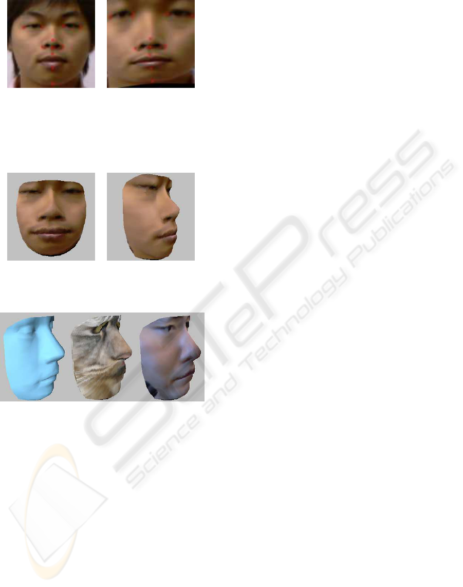
(a) (b)
Figure 1: Facial markers. (a) Facial markers v
i
on template
face. (b) Facial markers m
i
on 3D scan face.
Given a set of known displacements u
i
= v
i
− m
i
away from the 3D scan face positions at every marker
position i, construct a function that gives the displace-
ment u
j
for every non-constrained vertex j in the tem-
plate face model. We use a method based on radial
basis functions, that is the function of the form
f(v) =
∑
i
c
i
φ(k v− v
i
k) + Mv+ t (1)
where φ(r) are radially symmetric basis functions. M
and t are affine components. To determine the co-
efficient c
i
and the affine components M and t, we
solve a set of linear equations that include the interpo-
lation constraints u
i
= f(v
i
), as well as the constraints
∑
c
i
= 0 and
∑
c
i
v
T
i
= 0, which remove affine contri-
bution from the radial basis functions. Many different
functions for φ(r) have been proposed. We have cho-
sen φ(r) = |r|
2
log(|r|) for our function. We have ap-
plied this interpolation for each coordinate, X, Y, and
Z.
(a) (b)
Figure 2: Scattered data interpolation. (a) Original template
face. (b) Template face after RBF interpolation.
4.2 Model Data Fitting Optimization
After fitting roughly by scattered interpolation
method described above. We improve the quality of
fitting by minimizing the fitting error metric by adapt-
ing Allen’s method (Allen et al., 2003). We describe
BIOSIGNALS 2008 - International Conference on Bio-inspired Systems and Signal Processing
232

this method for fitting template face model to 3D scan
face. Each vertex v
i
in the template surface is influ-
enced by a 3x4 affine transformation matrix T
i
. We
try to find a set of transformations that move all of the
points in the template face to 3D scan face surface.
The quality of the match is evaluated using a set
of error functions: data error, smoothness error, and
marker error. These error terms are described in the
following sections.
Marker error. Equal number of Facial feature
points are placed on both the template face and the
3D scan face at the locations which are characteristic
for faces. About 13-20 features markers are suffice
to locate facial feature locations. We call the 3D lo-
cation of the markers on the 3D scan face m
1...m
, and
the correspondingvertex index of markers on the tem-
plate face t
1...m
. The marker error term E
m
minimizes
the distance between each marker’s location on the
template face and the 3D scan face:
E
m
=
∑
m
i=1
k T
t
i
v
t
i
− m
i
k
2
(2)
Data error. We fit the marker first, then fit all the
remaining points in the template face. We define a
data error term E
d
as the sum of the squared distances
between each vertex in the template face and the 3D
scan face surface.
E
d
=
∑
n
i=1
δ
i
dist
2
(T
i
v
i
,D) (3)
where n is the number of vertices in template face,
δ
i
is a weighting term to control the validity of the
match, and the dist() function computes the distance
to the closest point on the 3D face scan. If the surface
normals at the corresponding points are more than
90
◦
, set δ
i
to 0 otherwise set to 1.
Smoothness error. Allen (Allen et al., 2003) sug-
gested that simply moving each vertex in the template
face to its closest point in the 3D scan separately will
not result in a well arranged mesh, because neighbor-
ing parts of the template face could be mapped to dis-
parate parts of the 3D scan face. To constraint the
problem, we adopted the smoothness error, E
s
(Allen
et al., 2003). we formulate the constraint between ev-
ery two points that are adjacent in the template face:
E
s
=
∑
{i, j|{v
i
,v
j
}∈edges(T)}
k T
i
− T
j
k
2
F
(4)
where k · k is the Frobenius norm. By minimizing E
s
we prevent adjacent parts of the template face from
begin mapped to disparate parts of the 3D scan face.
Combining each error. Our complete objective
function E is the weighed sum of the three error func-
tions above:
E = αE
m
+ βE
d
+ γE
s
(5)
where the weights α, β, and γ are adjusted to guide
the optimization. We use a quasi-Newtonian solver,
L-BFGS-B (Zhu et al., 1994).
We first run the optimization using the relatively
low resolution mesh of the template face compared
with the 3D scan face. After that we subdivide the
resulting template face by inserting a new vertex be-
tween every edges of the mesh. Newly inserted vertex
position and its affine transformation is interpolated
between the two vertices of the edge.
We vary the weights, α, β, and γ, so that marker
point fits first then the remaining vertice move to the
appropriate position so that overall surface of the tem-
plate face fit to the 3D scan face. We run our optimiza-
tion as following
At the first stage (Low resolution of the template
face)
1. Fit the markers first: α=10, β=1, γ=1
2. Make the data error term to dominate: α = 1, β=10,
γ=1
At the second stage (High resolution of the tem-
plate face)
1. Continue the optimization: α=5, β=1, γ=0
2. Make the data error term to dominate: α = 0, β=10,
γ=1
Template face after fitting sometimes have ripple
over high curvature area. We have applied laplacian
smoothing (Taubin, 1995) to this surface and get
more smooth surface as seen in Fig 4.
(a) (b)
Figure 3: Fitting template face. (a) Template face after fit-
ting to 3D face scan. (b) Subdivided template face after
fitting.
A NOVEL TEMPLATE HUMAN FACE MODEL WITH TEXTURING
233

(a) (b)
Figure 4: (a)Smoothing face model after fitting. (b) display
in shading mode.
(a) (b)
Figure 5: (a)Fitted template face from another angle. (b)
Target 3D face scan from the same angle.
5 CONSTRAINED FACIAL
TEXTURE MAPPING
We propose a method based on radial basis function
(RBF) technique to apply a facial texture image to our
template based 3D face model. Fist we calculate the
mapping from 3D template face surface to 2D param-
eter space. With this mapping we obtain the template
face image. Then user specifically assigns the cor-
responding 2D points in the sample facial image to
those points in the template face image. We employ
RBF to morph the sample face image with the con-
straint of these feature points. Our method is charac-
teristic in that we do not re-calculate the 2D mapping
parameter for each face model, but use the common
parameterization prepared in-advance with the mor-
phed face image.
5.1 Template Face Image
Texture mapping or parameterization of 3D mesh is to
compute a mapping between a discrete surface patch
and an isomorphic planner mesh through a piecewise
linear mapping. This piecewise linear mapping is
simply defined by assigning each mesh node a pair
of coordinate (u,v) referring to its position on the
planer region. A number of work on parameterization
has been published, and almost all techniques explic-
itly aim at producing least-distorted parameterization.
We employ the intrinsic parameterizations (Desbrun
et al., 2002) for our parameterization method. Sum-
mary of the intrinsic parameterization is described in
Appendix. Fig 6 shows the result when we apply this
parameterization to our template face model. We call
the resulting 2D image the template face image.
(a) (b)
(c)
Figure 6: (a)3D template face. (b) 2D parameterization. (c)
template face image.
5.2 Face Image Morphing
2D image Morphing method we employ is basically
same as 4.1. The energy-minimization characteristic
of RBF ensures that the mapping function smoothly
interpolates constraints with non-deformation proper-
ties. User manually assign corresponding 2D points
in the sample texture image. User can set an arbitrary
set of constrained points, although for simplicity this
could be the same set of facial feature points as we
use in 4.1. The morphing result is in Fig 7. We trans-
form this morphed face image over the face model af-
ter fitting in Fig 8. Fig 9 shows various texture image
applied to our template face model.
6 CONCLUSIONS
We have succeeded to make face models which have
full point correspondence among them by fitting the
generic template face model to each 3D face scan. Al-
though initially it requires human interaction to locate
facial feature markers on each model, fitting process
BIOSIGNALS 2008 - International Conference on Bio-inspired Systems and Signal Processing
234

(a) (b)
Figure 7: Locate facial feature points int the original tex-
ture image which correspond to the facial feature points of
the template face image in Fig 6 (c). We then apply RBF
based image morphing with the constrained feature points.
(a)original texture image. (b) morphed texture image.
(a) (b)
Figure 8: Texture mapping after fitting. (a)textured face
model. (b) view from another angle.
Figure 9: Various texture mapping to template face model.
proceeds automatically. The resulting face model is
nicely fitted to the target 3D scan face. Although the
fitted face surface sometime is not as smooth as we
desire, we can smooth the surface by using laplacian
smoothing method without blurring the facial feature
points. Since our template face is created by ad-hoc
method, it calls for the way to create a ideal template
face. Praun et al (Praun et al., 2001) create a base do-
main model by tracing patch boundaries to represent
overall shape of the model. Although created base do-
main is too abstract for our template model, it could
be generated from its base domain. In stead of using a
triangular mesh, several studies have been made to fit
a spline surface over dense polygon mesh or points.
Besides of the patch boundary issue relating to spline
surfaces, it is a more suitable model for animation and
provide a fine but more expensive model for render-
ing.
Since we have a face model with consistent pa-
rameterization, it is a simple application to morph be-
tween any two faces. Although our face model after
fitting looks very similar to the original scan face, we
haven’tevaluated how accurate the fitting is. One pos-
sible method is to construct a graph which consists of
geodesic paths between every pair of the facial marker
points. The accuracy of the fitting could be done by
comparing these graphs.
We suggested one method to map texture image
over our template based face model. With this method
user doesn’t have to adjust texture coordinate for each
different face model, but rather morph the image with
the constraint of matched feature points between the
template face image and itself. For the restricted do-
main as human face model this method was found to
produce pleasing result.
REFERENCES
Allen, B., Curless, B., and Popovic, Z. (2003). The space of
human body shapes. In International Conference on
Computer Graphics and Interactive Techniques. ACM
SIGGRAPH.
Blanz, V. and Vetter, T. (2003). Face recognition based on
fitting a 3d morphable model. In IEEE Transactions
on Pattern Analysis and Machine Intelligence.
Desbrun, M., Meyer, M., and Alliez, P. (2002). Intrinsic
parameterization of surface meshes. In Eurographics
2002, Computer Graphics Proceedings. Eurograph-
ics.
Ekman, P. and V.Friesen, W. (1975). Unmasking the Face.
A guide to recognizing emotions from facial clues.
Prentice-Hall.
MINOLTA, K. (1999). Non-contact 3d laser scanner.
http://se.konicaminolta.us/products/3dscanners/
index.html.
Parke, F. I. (1972). Computer generated animation of faces.
In Proceedings ACM annual conference.
Praun, E., Sweldens, W., and Schr¨oder, P. (2001). Con-
sistent mesh parameterizations. In SIGGRAPH 2001,
Computer Graphics Proceedings. ACM Press / ACM
SIGGRAPH.
Taubin, G. (1995). A signal processing approach to fair
surface design. In Computer Graphics.
Vlasic, D., Brand, M., Pfister, H., and Popovic, J. (2005).
Face transfer with multilinear models. In ACM Trans-
actions on Graphics.
Zhu, C., Byrd, R., Lu, P., and Nocedal, J. (1994). Lbfgs-b:
Fortran subroutines for large-scale bound constrained
optimization. In LBFGS-B: Fortran subroutines for
large-scale bound constrained optimization, Report
NAM-11, EECS Department.
A NOVEL TEMPLATE HUMAN FACE MODEL WITH TEXTURING
235

APPENDIX
Parameterization of 3D mesh is to compute a map-
ping between a discrete surface patch and an isomor-
phic planar mesh with least distortion. Desbrun at el
(Desbrun et al., 2002) describe a general distortion
measure E, which is given by Dirichlet Energy E
A
and
Chi Energy E
χ
E = λE
A
+ µE
χ
where λ and µ are two arbitrary real constants.
E
A
=
∑
edges∈(i, j)
cotα
ij
|u
i
− u
j
|
2
where |u
i
− u
j
| is the length of the edge(i, j) in the
parameter domain, and α
ij
is the opposite left angle
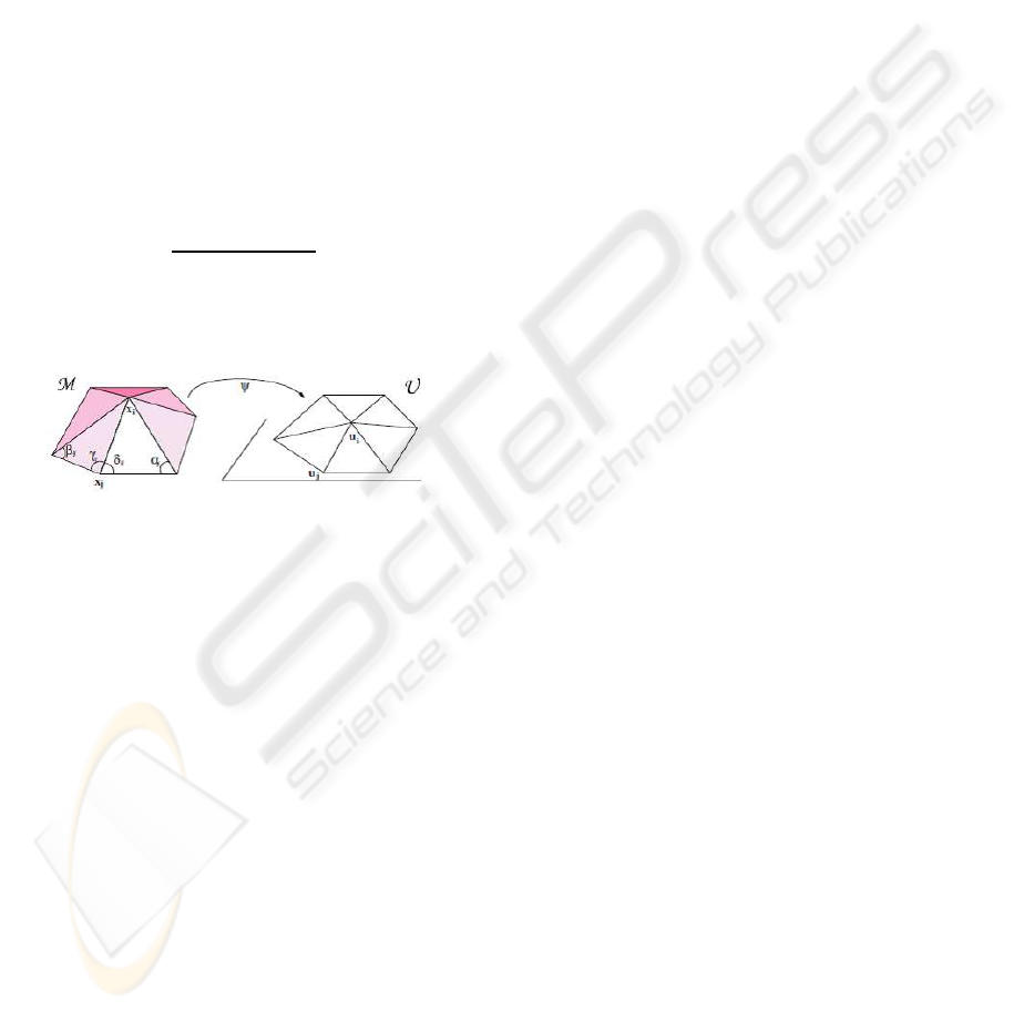
in 3D as shown in Fig 10.
E
χ
=
∑
j∈N(i)
(cotγ
ij
+ cotδ
ij
)
|x
i
− x
j
|
2
(u
i
− u
j
)
2
where the angles γ
ij
and δ
ij
are define in Fig 10.
Figure 10: 3D 1-ring and its associated flattened version.
Since the gradient of E is linear, computing a pa-
rameterization reduces to solving the following sparse
linear system:
MU =

λM
A
+ µM
χ
0 I

U
internal
U
boundary

=

0
C
boundary

= C
where U is the vector of 2D-coordinates to solve
for. C is a vector of boundary conditions that contains
the positions where the boundary vertices are placed.
M
A
and M
χ
are sparse matrices where coefficients are
given respectively by:
M
A
ij
=





cot(α
ij
) + cot(β
ij
) if j ∈ N(i)
−
∑
k∈N(i)
M
A
ik
if i = j
0 otherwise,
M
χ
ij
=





(cot(γ
ij
) + cot(δ
ij
))/|x
i
− xj|
2
if j ∈ N(i)
−
∑
k∈N(i)
M
χ
ik
if i = j
0 otherwise,
BIOSIGNALS 2008 - International Conference on Bio-inspired Systems and Signal Processing
236