ADAPTIVE IMAGE RESTORATION USING A LOCAL NEURAL
APPROACH
I. Gallo, E. Binaghi and A. Macchi
Universita’ degli Studi dell’Insubria, via Ravasi 2, Varese, Italy
Keywords:
Image restoration, gradient descent, neural networks.
Abstract:
This work aims at defining and experimentally evaluating an iterative strategy based on neural learning for
blind image restoration in the presence of blur and noise. A salient aspect of our solution is the local esti-
mation of the restored image based on gradient descent strategies able to estimate both the blurring function
and the regularized terms adaptively. Instead of explicitly defining the values of local regularization param-
eters through predefined functions, an adaptive learning approach is proposed. The method was evaluated
experimentally using a test pattern generated by a function checkerboard in Matlab. To investigate whether
the strategy can be considered an alternative to conventional restoration procedures the results were compared
with those obtained by a well known neural restoration approach.
1 INTRODUCTION
Restoring an original image, when given the degraded
image, with or without knowledge of the degrading
point spread function (PSF) or degree and type of
noise present is an ill posed problem (Andrews and
Hunt, 1977) and can be approached in a number of
ways (Sezan and Tekalp, 1990).
Iterative image restoration techniques often at-
tempt to restore an image linearly or nonlinearly by
minimizing some measure of degradation such as
maximum likelihood (Andrews and Hunt, 1977), or
constrained least square error (Gonzalez and Woods,
2001), by a wide variety of techniques. Generally the
image degradation model suitable for most practical
purposes is formed as a linear process with additive
noise for which the matrix form is
g = Hf+ n (1)
Where g and f are the lexicographically ordered de-
graded and original vectors respectively, H is the
degradation matrix, and n represents the noise. The
aim of image restoration algorithms is to find an es-
timate that closely approximates the original image f,
given g.
Blind restoration methods which attempt to solve
the restoration problem without knowing the blurring
function is of great interest in many important appli-
cation domains, such as biomedical imaging, charac-
terized by a rapid evolution of imaging devices. In
blind methods, both the degradation matrix and the
original image are unknown, making the problem dif-
ficult to solv based on the observed image only. Many
methods have been devised to find these two com-
ponents by incorporating properly specified knowl-
edge (or constraints) (Kundur and Hatzinakos, 1996).
However the use of various stringent constraints for
insufficient information in the deconvolution process
limits the applications of these methods. In the pres-
ence of both blur and noise, the restoration process re-
quires the specification of additional smoothness con-
straints on the solution. This is usually accomplished
in the form of a regularization term in the associated
cost function (Katsaggelos, 1991)
Regularized image restoration methods aim to
minimize the constrained least-squares error measure
E =
1
2
kg− H
ˆ
fk
2
+
1
2
λkD
ˆ
fk
2
(2)
where
ˆ
f is the restored image estimate, λ represents
the regularization parameter and D is the regulariza-
tion matrix. A small parameter value, which deem-
phasizes the regularization term, implies better fea-
ture preservation but less noise suppression for the
161
Gallo I., Binaghi E. and Macchi A. (2007).
ADAPTIVE IMAGE RESTORATION USING A LOCAL NEURAL APPROACH.
In Proceedings of the Second International Conference on Computer Vision Theory and Applications - IFP/IA, pages 161-164
Copyright
c
 SciTePress

restored image, whereas a large value leads to better
noise suppression but blurred features.
The aim of this work is to define and experimen-
tally evaluate an iterative strategy based on neural
learning for blind image restoration in the presence
of blur and noise. A salient aspect of our solutions
is the local estimation of the restored image based
on gradient descent strategies able to estimate both
the blurring function and the regularized terms adap-
tively. Instead of explicitly defining the local regu-
larization parameters values through predefined func-
tions, an adaptive learning approach is proposed. The
neural learning task can be formulated as the search
for the most adequate restoration parameters related
to blurring function and regularization term, through
the supply of appropriate local/contextual training ex-
amples.
Experiments were conducted using synthetic im-
ages for which blur functions and original images are
completely known.
2 RESTORATION AS A
NEURAL-NETWORK
LEARNING PROBLEM
This work proposes an iterative method which uses
gradient descent algorithm to minimize a local cost
function derived from traditional global constrained
least square measure (Eq. 2). We call this method
Local Adaptive Neural Network (LANN).
The degradation measure we consider minimiz-
ing is a local cost function E
x,y
defined for each pixel
(x,y) in a MxN image:
E
x,y
=
1
2
[g
x,y
− h∗
ˆ
f]
2
+
1
2
λ[d ∗
ˆ
f]
2
(3)
where h ∗
ˆ
f denotes the convolution computed in a
point (x,y).
The blur function h(x, y) is defined as a bivariate
Gaussian function:
h(x,y) =
1
2πσ(w
x
)σ(w
y
)
e
−
1
2
((
x
σ(w
x
)
)
2
+(
y
σ(w
y
)
)
2
)
(4)
where the parameters σ(w
x
) and σ(w
y
) are functions
whose values represent standard deviations in the
range [m,n]:
σ(x;m,n) =
n− m
1+ e
−a(x−c)
+ m (5)
and a and c are logistic function’s slope and off-
set respectively. The parameter λ(w
λ
) is a function
whose values represent regularization terms in the
range [0,1]
λ(x) =
1
1+ e
−x
(6)
The range [0, 1] is suggested by Katsaggelos and
Kang (A. K. Katsaggelos, 1995).
An adaptive neural learning procedure is defined
including a non-conventional sub-goal formulated as
the search for the most adequate blurring filter size
and/or regularization term acting on w
x
, w
y
and w
λ
respectively. Weight updating is performed based on
contextual information drawn from a window cen-
tered on the current pixel and having dimension W =
⌈3σ
x
⌉2+ 1 and H = ⌈3σ
y
⌉2+ 1.
The restoration algorithm is described in the fol-
lowing (Algorithm 1).
Algorithm 1 Calculate
ˆ
f,σ
x
= σ(w
x
),σ
y
= σ(w
y
) and
λ(w
λ
).
Require: Scale each pixel of the original gray level
blurred image using (1/2
b
− 1) as scale factor (b is
the number of bits in each pixel of g image)
Require: Initialize w
x
, w
y
and w
λ
to some small ran-
dom value
Require: Initialize
ˆ
f with random values in the range
[0.1,0.9]
repeat
for x = 1 to M; y = 1 to N do
select the pixel (x,y);
compute the new width W and height H of the
gaussian kernel;
compute each partial derivative:
∂E
x,y
∂
ˆ
f
s,t
,
∂E
x,y
∂w
x
,
∂E
x,y
∂w
y
,
∂E
x,y
∂w
λ
(7)
update each parameter as follow:
ˆ
f
t
x,y
,w
t
x
,w
t
y
,w
t
λ
(8)
end for
until (|
ˆ
f
t
x,y
−
ˆ
f
t−1
x,y
| < ε, ∀(x,y))
To facilitate the algorithm convergence the re-
stored image estimate
ˆ
f must be initialized with ran-
dom values in the range [0,1] obtaining scaling origi-
nal intensity values.
In principle the algorithm is conceived to estimate
simultaneously both the blurring function and the reg-
ularization term acting as a complete blind deconvo-
lution method.
The present work investigates experimentally the
potentialities and/or limits of the proposed algorithm
coping with the restoration task at increasing levels

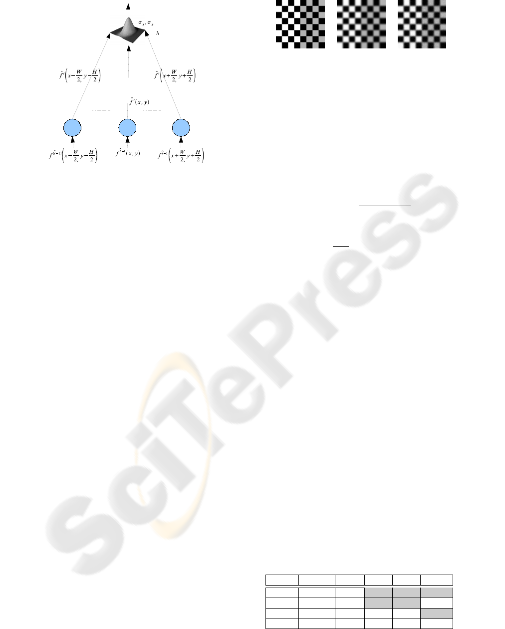
Figure 1: Graphic Representation of the proposed LANN
Model.
of complexity, i.e. with or without prior knowledge
of the blurring function and/or statistics of additive
noise.
3 EXPERIMENTS
The method was experimentally evaluated and com-
pared using a test image 64x64 generated by checker-
board function in Matlab (Gonzalez et al., 2003) (Fig.
2a).
Several experiments were conceived and con-
ducted with the aim of evaluating restoration accuracy
under different degradation conditions.
The experiment heuristically assessed the follow-
ing parameter values: allowing standard deviations
min and max values: n = 3.0 and m = 0.2; ε value for
stop condition: 0.0001; w
λ
is initialized to a random
value in the interval[−0.1, 0.1]; w
x
and w
y
are initial-
ized to a random value in the interval[−0.6,−0.5].
3.1 Restoration in the Absence of Noise
For these experiments the image was blurred using
a Gaussian filter having σ
x
= σ
y
= 1 (Fig. 2b) while
the learning parameters were fixed at η = 0.9 and α =
0.5.
Initially the algorithm was run having fixed all the
parameters.
In a second experiment the algorithm was run hav-
ing fixed the internal parameters related to σ
x
and σ
y
and varying the parameter related to λ adaptively.
Next the restoration algorithm was run having
fixed the internal parameter related to λ and varying
parameters related to σ
x
and σ
y
adaptively.
(a) (b) (c)
Figure 2: Original (a), blurred with σ
x
= 1 and σ
y
= 1 (b);
blurred image plus Gaussian noise (σ = 5) (c).
Finally the algorithm was run varying all the pa-
rameters adaptively, while in the last experiment all
the parameters were fixed.
To evaluate the restoration performance of our
approach quantitatively ISNR and RMSE measures
were adopted. These can be estimated as follows:
ISNR = 10log
10
{
∑
MN
i=1
( f
i
− g
i
)
∑
MN
i=1
(
ˆ
f
i
− f
i
)
} (9)
RMSE = (
1
MN
MN
∑
i=1
(
ˆ
f
i
− f
i
)
2
)
1/2
(10)
Results obtained are summarized in Table 1.
When applied under favorable conditions of absence
of noise, the restoration algorithm shows a good be-
havior confirming the feasibility of the approach. In-
creasing the number of free parameters during learn-
ing the algorithm shows a stable behavior with less
difference among performances.
3.2 Restoration in the Presence of Noise
For these experiments the image, blurred using a
Gaussian filter having σ
x
= σ
y
= 1, was corrupted by
Gaussian noise having standard deviation σ = 5(Fig.
2c). The learning parameters were fixed at η = 0.01
and α = 0.5.
Initially the algorithm was run having fixed all the
parameters.
In a second experiment the algorithm was run hav-
ing fixed the internal parameters related to σ
x
and σ
y
and varying the parameter related to λ adaptively.
In a third experiment the restoration algorithm was
run having fixed the internal parameter related to λ
Table 1: Results obtained restoring the image shown in Fig.
2b using the proposed LANN model. The grey cells contain
fixed parameters.
ISNR RMSE time σ
x
σ
y
λ
11.61 11.91 272s 1.0 1.0 0.0
12.68 11.0 261s 1.0 1.0 0.001
9.68 14.88 316s 0.97 0.95 0.0
8.31 17.42 300s 0.96 0.92 0.002

(a) (b) (c) (d)
Figure 3: Restoration results in the absence of noise: (a) re-
sult by LANN with all parameters fixed; (b) result by Hop-
field. Restoration results in the presence of noise: (c) result
by LANN with all parameters fixed; (d) result by Hopfield.
and varying parameters related to σ
x
and σ
y
adap-
tively.
In the last experiment the algorithm was run lay-
ing to vary adaptively all the parameters.
Results obtained are summarized in Table 2.
Under noisy conditions the algorithm registered a
decrease in performances evaluated both using ISNR
and RMSE indexes for all four cases examined. The
behavior is again quite stable, even if a slight decrease
in performance was recorded in cases in which blur
filter size was free to vary.
3.3 Comparison Analysis
The proposed method was compared with the
neural restoration method proposed by Zhou et
al. (Y.T. Zhou, 1988) based on the Hopfield model.
Results obtained in non-noisy and noisy conditions
are reported in Table 3. Consistently with the LANN
method performances are superior in the case of
non noisy conditions. Comparing results in Table 3
with those present in the first rows of Tables 1 and
2, our method prevails under non noisy conditions,
whereas the Hopfield-based method yielded better
performances under noisy conditions.
Visual inspection of images restored by the two
methods in Fig. 3 highlights perceptual differences.
The image restored by the LANN method lacks the
ringing effect that is evident in the other image near
the boundary; the image produced by the Hopfield
based method appears more smoothed. Focusing on
the right half image produced by the LANN method,
some artifacts in the gray squares, probably related to
initialization conditions, are evident.
Table 2: Results obtained restoring the image shown in Fig.
2c using the proposed LANN model. The grey cells contain
fixed parameters.
ISNR RMSE time σ
x
σ
y
λ
3.38 30.92 592s 1.0 1.0 0.0004
3.61 30.09 586s 1.0 1.0 0.06
1.46 38.56 418s 0.82 0.81 0.0004
1.51 38.34 393s 0.81 0.80 0.14
4 CONCLUSION
The objective of this work was a preliminary exper-
imental investigation into the potentialities of a new
restoration method based on neural adaptive learning.
Results obtained demonstrate the feasibility of the
approach. Limitations of the method in terms of
restoration quality and computational complexity are
evident dealing with noisy images.
Further investigations and improvements of the
method are planned focusing on faster neural learn-
ing, initialization conditions and robustness in han-
dling different levels of noise.
REFERENCES
A. K. Katsaggelos, M. G. K. (1995). Spatially adaptive it-
erative algorithm for the restoration of astronomical
images. Int. J. Imaging Syst. Technol., 6:305–313.
Andrews, H. C. and Hunt, B. R. (1977). Digital Image
Restoration. Prentice Hall Professional Technical Ref-
erence.
Gonzalez, R. C. and Woods, R. E. (2001). Digital Im-
age Processing. Addison-Wesley Longman Publish-
ing Co., Inc., Boston, MA, USA.
Gonzalez, R. C., Woods, R. E., and Eddins, S. L. (2003).
Digital Image Processing Using MATLAB. Prentice-
Hall, Inc., Upper Saddle River, NJ, USA.
Katsaggelos, A. K. (1991). Digital Image Restoration.
Springer-Verlag New York, Inc., Secaucus, NJ, USA.
Kundur, D. and Hatzinakos, D. (1996). Blind image decon-
volution. IEEE Signal Processing Magazine, 13:43–
64.
Sezan, M. I. and Tekalp, A. M. (1990). Survey of recent de-
velopments in digital image restoration. Optical En-
gineering, 29:393–404.
Y.T. Zhou, R. Chellappa, B. J. (1988). Image restoration
using a neural network. IEEE Trans. Acoust,. Speech,
Sign. Proc., 36:38–54.
Table 3: Results obtained restoring the images shown in
Fig. 2b-c using the Hopfield model proposed by Zhou. The
grey cells contain fixed parameters.
ISNR RMSE time σ
x
σ
y
λ
7.827 18.417 323 s 1.0 1.0 0.0
4.97 25.73 264s 1.0 1.0 0.0004