RECONSTRUCTING WAFER SURFACES WITH MODEL BASED

SHAPE FROM SHADING

Alexander Nisenboim

Israel Institute of Technology, Applied Mathematics Dept., Haifa, Israel

Alfred Bruckstein

Israel Institute of Technology, Comuter Science Dept., Haifa, Israel

Keywords:

Shape from shading, wafer, scanning electron microscope, mathematical model, wavelets, non-linear opti-

mization.

Abstract:

Model based Shape From Shading (SFS) is a promising paradigm introduced by J. Atick for solving such

inverse problems when we happen to have some prior information on the depth proﬁles to be recovered. In the

present work we adopt this approach to address the problem of recovering wafer proﬁles from images taken

by a Scanning Electron Microscope (SEM). This problem arises naturally in the microelectronics inspection

industry. A low dimensional model based on our prior knowledge of the types of depth proﬁles of wafer

surfaces has been developed and based on it the SFS problem becomes an optimal parameter estimation.

Wavelet techniques were then employed to calculate a good initial guess to be used in Levenberg-Marguardt

(LM) minimization process that yields the desired proﬁle parametrization. The proposed algorithm has been

tested under both Lambertian and SEM imaging models.

1 INTRODUCTION

The problem of recovering a 3D object’s shape from

its shaded image, namely the Shape From Shading

(SFS) problem, has intrigued the computer vision re-

searchers for more then 30 years. The research in this

area was mostly inspired by the fact that our brain has

an outstanding ability to perceive the depth of the ob-

served scene from 2D images on the retina. Shading

is only one of the clues used by our brain to do the job.

It is interesting that despite the lack of our understand-

ing of this cognitive feature and major difﬁculties of

our mathematical modeling attempts, nowadays there

is a need for SFS-based applications in some branches

of the computer industry. Manufacturing of integrated

circuit wafers is an expensive and delicate process

and a great deal of effort is invested in the control of

quality and acceptability of such crucial device fea-

tures as contact holes, tracks etc. Typically, the man-

ufacturers are interested in measuring the geometri-

cal parameters of the features and due to the ”nano-

sizes” of the structures studied, the non-destructive

Low-Voltage SEM is used. Thus, the necessity of

3D-surface measurements from 2D SEM images nat-

urally arises. The very nature of the SFS idea is to

exploit the fact that the variations of surface’s orien-

tation cause the variations of the brightness at corre-

sponding areas in the image. However, the brightness

only carries information about the projection of sur-

face normal on the light source direction (see eq. (1)

) and hence the surface normal at each point cannot

be uniquely discovered. Thus, mathematically speak-

ing, the SFS problem appears to be ill-posed, however

recent interesting reformulations challenge this view-

point (Prados et al., 2004). One way to overcome

these fundamental difﬁculties is to reformulate the

SFS as a variational problem while introducing reg-

ularization terms into the minimized functional (Horn

and Brooks., 1986), (Zheng and Chellappa, 1991).

There are also alternative general approaches using

facet model (T. Pong and Shapiro., 1989), level sets

(R. Kimmel and Bruckstein., 1995) or hierarchical

representations (A. Jones, 1994). However, being

general, these approach could suffer from some draw-

backs (A. Jones, 1994). In this work, following a

paradigm introduced by J. Atick (Atick et al., 1996),

we try to directly use a priori information about the

geometry of the studied surfaces. Giving up gener-

333

Nisenboim A. and Bruckstein A. (2007).

RECONSTRUCTING WAFER SURFACES WITH MODEL BASED SHAPE FROM SHADING.

In Proceedings of the Second International Conference on Computer Vision Theory and Applications - IU/MTSV, pages 333-340

 SciTePress

ality, we assume a model of the surface controlled

by a ﬁnite set of parameters. The resulting para-

meter estimation SFS problem appears to be simpler

than the original one. The initial estimates are ob-

tained by means of analysis of the wavelet decom-

position of the given image and subsequently a para-

meter ﬁtting process is carried out. Finally, an itera-

tive LM minimization procedure has been adopted in

our work in order to insure stable numerical conver-

gence. It should be mentioned here that this research

was initiated and partially sponsored by Applied Ma-

terials,Inc., so the real data is banned from being pub-

lished due to its high business sensitivity. Therefore

the whole method is explained using a synthetic but

illustrative example. This paper is organized as fol-

lows. In Section 2 we mathematically formulate the

SFS problem and brieﬂy overview the previous rele-

vant work. Section 3 contains the description of the

new method. Section 4 presents results and discus-

sion.

2 THE SHAPE FROM SHADING

PROBLEM

2.1 General Problem Setup

The monocular SFS problem is deﬁned as follows.

Suppose we are looking for a smooth height ﬁeld

z = z(x,y) over region D ⊂ R

, and we are given its

shaded image I(x,y). The value of I at each point

depends on reﬂectance properties of the surface, its

gradient and imaging geometry parameters like light

direction e.t.c. This dependence is called a reﬂectance

function, and we denote it R = R(p,q), where p = z

and q = z

. The relationship

I(x, y) = R(p(x,y),q(x,y)) (1)

is called the irradiance equation and we state the SFS

problem as an attempt to recover the surface height

ﬁeld z(x,y) from a single shaded image I(x, y) given

the reﬂectance function R, i.e. to determine z(x,y) that

satisﬁes (1). Some assumptions are to be made about

imaging geometry. First, we assume that the size of

the studied object is small, compared to the viewing

distance, which enables us to presume orthographic

projection to the image plane. We also assume that

the camera direction coincides with the Z axis. In this

case one can choose the coordinate system of both

image and object planes to be identical and denoted

by (X,Y). We denote η to be composite albedo which

essentially captures the energy dissipation properties

of the surface. We assume that η is constant along the

surface. We also denote

L to be the unit vector of the

illumination direction. We assume that there is only

one source of light located at inﬁnity.

2.2 Imaging Models

By deﬁnition, if R(p,q) = η < ~n(x,y),

L > we say

that a surface exhibits Lambertian diffuse reﬂection

property. Here <,> is a standard inner product and

~n(x,y) = (−p,−q,1)/

+ q

+ 1 is a unit normal

vector to the surface. In case of SEM, the sim-

plest image formation model is given by R(p,q) =

η/<~n(x,y),

L >. This model holds well when spec-

imen is coated by gold and in absence of charging

artifacts (Reimer, 1993). It turns out that the prob-

lem of computing η and

L can be solved separately

(Zheng and Chellappa, 1991) and, therefore, we sup-

pose them to be known. We should note here that the

algorithm presented below in no way depends on any

particular imaging model.

2.3 Previous Work

The problem of SFS was stated by B. Horn in 70’s

(Horn, 1975). His ﬁrst solution involved characteris-

tic strips expansion of the irradiance equation (1) and

was not stable in practice due the noise sensitivity and

error accumulation problems. During 80’s, Horn and

others (Horn and Brooks., 1986), (Zheng and Chel-

lappa, 1991) reformulated the problem and solved it

using the calculus of variations. Nice and comprehen-

sive analysis of other SFS techniques can be found

in (Zhang et al., 1999). Another important idea was

suggested by J. Atick (Atick et al., 1996). In this

work the authors dealt with the problem of recovering

of the shape of human faces from their shaded images.

In order to employ the a priori information about the

class of objects studied, Atick gives up generality (of

the variational approach) and solves the SFS prob-

lem for this particular class. The exact laser scans of

200 faces represented in a cylindrical coordinate sys-

tem {r

(θ,l)}

200

i=1

where regarded as independent re-

alizations of some stochastic process. Thus a ”face-

surface” can be represented as

r(θ,l) = r

(θ,l) +

∑

i=1

(θ,l) (2)

where r

(θ,l) is a ”mean-face”, and u

(θ,l) are the

ﬁrst M components of Karhunen-Loeve decompo-

sition derived from the scanned surfaces, so-called

”eigen-faces”. So, denoting

α = (α

,α

,... ,α

) the

SFS problem can be reformulated as

min

∑

l,θ

(I(x(l,θ),y(l,θ)) − R(p, q;

α))

(3)

This basically means that we are looking for the best

coefﬁcients of the linear combination of the ”eigen-

faces” that explain our input image in terms of mean

square error. Thus the SFS problem becomes one of

optimal parameter estimation and it has been solved

using gradient descent method.

3 MODEL BASED SFS FOR

WAFERS

3.1 A Priori Knowledge

Unlike the work of J. Atick mentioned above, with

surfaces of wafers no statistical information is avail-

able. Therefore we concentrate our efforts to employ

a priori knowledge about wafer geometry in attempt

to work out low-dimensional and meaningful repre-

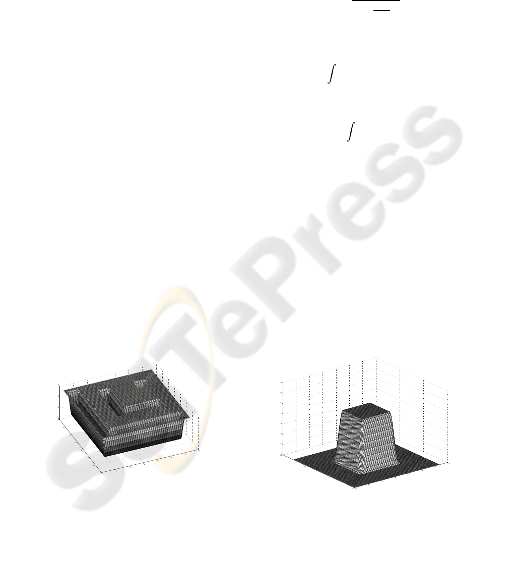
sentations of wafer surfaces. Wafer surface could be

characterized as a plane with a set of mutually dis-

joint contact holes and tracks (Figure 1) which should

subsequently be ﬁlled with conducting matter. These

tracks might be either straight or bent. One can as-

sume that the edges of holes and tracks are parallel to

the X and/or Y axes of the image plane. This assump-

tion does not always hold in practice, but its violation

is rather rare and hence disregarded in our model. The

shape of holes may vary with their size. Holes of rel-

atively large size look like a rectangle with somewhat

rounded corners and edges which are normally par-

allel to the axes. However, smaller holes assumed to

have rather rounded shape like ellipses or circles. One

cannot assume that slopes of holes and tracks are sym-

metrical. In the next section we deﬁne mathematical

objects which ﬁt well the geometry described above.

100

120

140

100

120

140

−1.5

−1

−0.5

Figure 1: Wafer surface.

3.2 Mesa Function

We start with the following formal construction of a

so-called mesa (table) function. Let us deﬁne

f(x;x

,ε) =











cexp

1−



x−x



, |x− x

| < ε

0 , elsewhere

(4)

The constant c in this deﬁnition is such that

+ε

−ε

f(x;x

,ε)dx = 1 (5)

Then a mesa function is then deﬁned as

F(x;x

,ε

) =

−∞

( f(t;x

,ε

) − f(t;x

,ε

))dt

(6)

The parameters of mesa function have simple geomet-

rical interpretation:

1. |x

− x

| is responsible for the size of the ”pulse”.

2. ε

,ε

control the slopes of the function.

Now, let us deﬁne 2D mesa function of height h to be

h times tensor product of two 1D mesa functions. For

simplicity we denote

= (x

,ε

);

= (y

,ε

)

α = (x

,ε

,h) = (

,h)

and then

T(x,y;

α) = h · F(x;

) · F(y;

)

See Figure 2.

100

120

140

100

150

0.2

0.4

0.6

0.8

1.2

1.4

Figure 2: 2D mesa function.

3.3 Surface Representation

By means of 2D mesa functions we can build success-

ful representations of surfaces of the type described

in the previous section. Indeed, a straight track or

hole feature can be represented as a negative 2D mesa

function. A bent track, for example, can be con-

structed as difference of two 2D mesa functions when

one of them is shifted from another. Therefore we can

write

z(x,y) =

∑

i=1

(x,y), (7)

when

(x,y) = T(x,y;

)

which means that in terms of this model, SFS prob-

lem becomes one of optimal parameter estimation. In

the following sections we shall develop a technique

to separate between the features and ﬁnd N initial sets

of parameters (along with N itself) for each feature

instead attempting to estimate them all together.

3.4 Strategy

It is well known that in order to succeed in the mini-

mization process mentioned above a good initial es-

timate is needed. Let us brieﬂy describe our main

strategy. It is very common practice to take into

account prior knowledge about image structure (like

edge-geometry, or statistics of the noise e.t.c.) to sim-

plify the very complex tasks of image processing and

analysis. In our case, the surface model implies a

certain geometrical structure of the image. First, all

edges are straight and parallel to the axes. Second,

the edges are expected to be organized in well-deﬁned

constellations. For example, in case of an image of

a relatively large contact hole, its edges will tend to

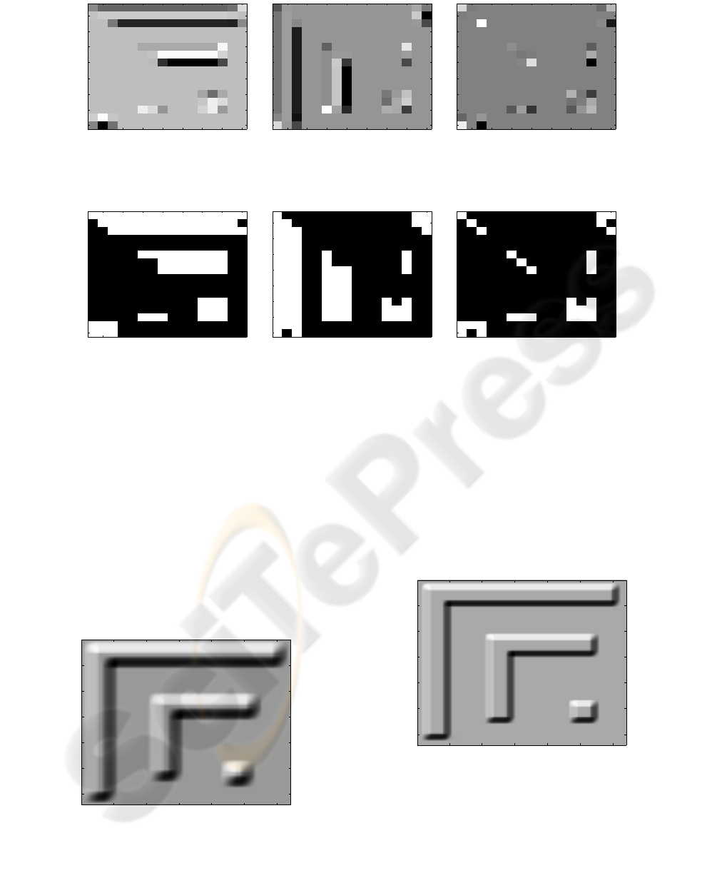
form a rectangular shape. See Figure 3. Therefore, by

decomposing the image in Haar wavelets basis, and

picking the largest amplitude coefﬁcients one can get

compact and effective representation of image singu-

larities. Moreover, large Haar coefﬁcients will carry

the spatial information of image singularities at each

level of the decomposition. Since image singularities

form well-organized clusters, so do the large ampli-

tude wavelet coefﬁcients.Thus the wavelets represen-

tation properties could be exploited in order to local-

ize every surface feature from its coefﬁcients cluster

and roughly calculate its parameter vector.This vector

will subsequently serve as the starting point for the

Least Square Error (LSE) optimization process and

iteratively reﬁned toward the ﬁnal result.

Two points are worth mentioning. First, applying this

strategy we will separate surface features and treat

20 40 60 80 100 120

100

120

Figure 3: Lambertian image of the surface shown on Fig-

ure 1.

them independently which solves the problem of un-

known number of terms in model (7). Second, the ini-

tial parameter estimates are geometrically meaningful

which signiﬁcantly reduces our chances to fall into

some local minima during the LSE procedure. Let us

elaborate on this strategy in the following sections.

3.5 Haar Wavelets for Tracking

Singularities

The expansion of I(x, y) ∈ L

) in the orthonormal

basis of Haar functions



j,n

,Ψ

j,n

,Ψ

j,n



j∈Z,n∈Z

I(x, y) =

∑

k=1

∞

∑

j= −∞

∑

j,n

(8)

where

j,n

f,Ψ

j,n

will be referred as Discrete Haar Transform (DHT)

and it has an interpretation in terms of image details

aggregation at all resolution levels that range from 0

to +∞, (Mallat, 1999). The inner products w

j,n

repre-

sent details in the horizontal direction, w

j,n

give the

details in vertical direction and w

j,n

are the details in

both directions (corners)(Fig. 4). It is suitable rec-

tangular shape of Haar functions which makes them

appealing to our model, since they should correlate

well with mesa functions.Suppose that at each res-

olution scale s three binary images H

, V

and D

are produced (Fig. 5). The images are built from

the large amplitude coefﬁcients corresponding to hor-

izontal, vertical and diagonal directions by means of

binarization process. For any binary image B we de-

note CC(B) = {CC

(B)} to be the set of connected

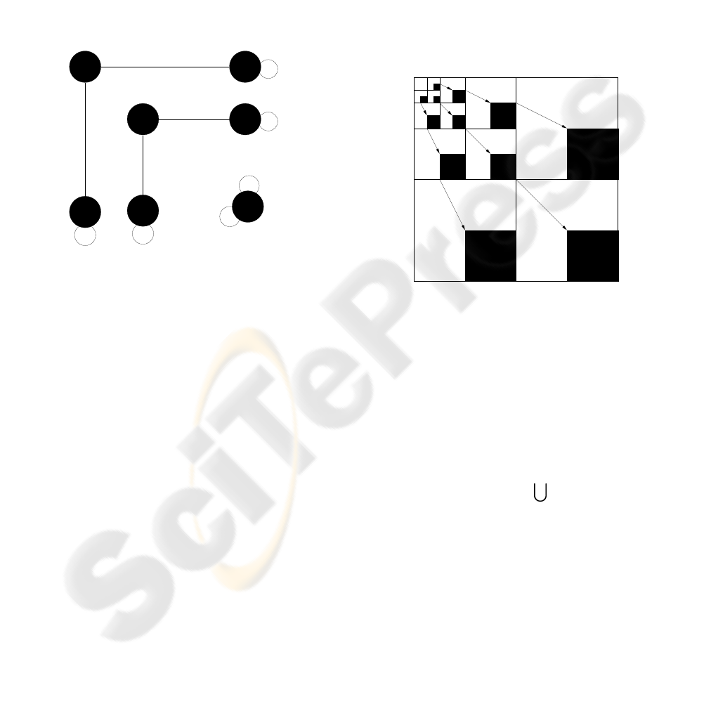
components of B. Then let us deﬁne a Feature Track-

ing Graph (FTG) G

using the following deﬁnitions:

1. The set of vertices of G

is equal to the set

CC(D

2. The unordered pair (v

) of vertices is said to

be H-type edge if

∃k : CC

) ∩CC

) 6= 0

and

) ∩CC

) 6= 0

or V-type edge if

∃k : CC

) ∩CC

) 6= 0

and

) ∩CC

) 6= 0

Figure 6: FTG built from the images illustrated on Fig 5.

Note that the operation ∩ should be redeﬁned here

because, CC

) and, for example,CC

) are em-

bedded in different images. One can imagine that H

and D

are placed ”one on top of the other”, or in

other words, they share the same coordinate system.

In this sense the operation ∩ is well deﬁned. Uncon-

nected FTG G

can be decomposed to the set of N

connected subgraphs G

= {CSG

)}

i=1

by means

of any standard method. Decomposition of FTG in

connected subgraphs naturally reﬂects the geometri-

cal structure of singularities at each level of reso-

lution. For each CSG

) it is possible to locate

the spatial position of the surface singularities which

originated the coefﬁcientsthatCSG

) is built from,

and hence the number N of connected subgraphs is

our estimate of number of terms in model (7). In or-

der to trace the location of surface features we need

a notion of the Spatial Orientation Trees (SOT) bor-

rowed from the work of Shapiro (Shapiro., 1986). In

this work so-called Zero Tree (ZT) have been used as

a tool to optimize the transformation coefﬁcients cod-

ing. Here we slightly modify ZT construction in order

to adopt it to our goals. For each spatial orientation

k = 1,2,3 we create quad-trees by relating recursively

each coefﬁcient at the scale s and position (p,q), say

(p,q), to its four children at the next, ﬁner, scale

s+ 1: w

s+1

(2p,2q),w

s+1

(2p + 1,2q),w

s+1

(2p,2q +

1),w

s+1

(2p + 1,2q + 1) Usually, the branching rule

of the coefﬁcients at the most coarse scale, say s = 0,

is different. Each coefﬁcient w

(p,q) is associated

with the three wavelet coefﬁcients at the same scale

and location: w

(p,q), w

(p,q), and con-

sidered to be the roots of the trees.We artiﬁcially at-

tach the image planes to each spatial orientation. The

reason behind it is that we are going to use not the val-

ues of the pixels, but only their absolute coordinates.

The ”pseudo-coefﬁcients”at this artiﬁcial level on the

image plane will be considered as the leaves of the

trees. The construction of SOT is illustrated in Fig-

ure 7. Note that if at some scale level s and position

Image Plane Image Palne

Image Plane

S = 0

S = 1

S = 2

S = 3

ROI

ROIROI

Figure 7: Spatial Orientation Tree.

(p,q) there is a wavelet coefﬁcient w

(p,q) of high

amplitude, then all image singularities which possibly

contributed to the coefﬁcient are likely to be included

into the spatial area of the leaves of the SOT rooted at

(s, p,q). Let us denote it as the region of inﬂuence of

(s, p,q) by ROI(s, p,q), see Figure 7. Clearly, the

wavelet coefﬁcients w

(p,q), w

(p,q) and w

(p,q)

have the same ROI. Now, the ROI of each connected

subgraph can be deﬁned as

ROI(CSG

)) =

(p,q)∈P

)

ROI(s, p,q) (9)

where P

) is the set of all points in H

, V

and D

which constitute the connected subgraph CSG

One can also see that by construction of the SOT the

ROI’s of two different points (s, p

) and (s, p

)

are disjoint, and hence so are the ROI’s of two differ-

ent connected subgraphs. Thus, the decomposition of

the graph G

to the mutually disjoint connected sub-

graphs enables us to deﬁne a set of mutually disjoint

domains on the image plane where the potential sur-

face features are located. Then, it is possible to calcu-

late the set of the initial guesses for the feature loca-

tion in order to initialize the optimization process.We

2 4 6 8 10 12 14 16

(H) (V) (D)

Figure 4: One scale of HDT of the image on Fig. 3.

2 4 6 8 10 12 14 16

Figure 5: Binarization of the images displayed of Fig. 4.

use a rather simple strategy to establish the initial es-

timates for the surface parameters. Given the sets of

mutually disjoint connected subgraphs and their ROIs

we apply the following two-step heuristic decision:

S 1: Decide on the type of the feature (track/hole). For

example, number of vertices and types of edges of

CSG

) could be used.

S 2: Given the ROI, try to compute the parameters of

a symmetrical feature of an appropriate type such

that it would fully occupy the ROI. See Fig. 8.

20 40 60 80 100 120

100

120

Figure 8: Image of the initial guess.

The only parameter which does not play any role in

this heuristic decision is the parameter h of the 2D

mesa-function. We suggest to overcome this prob-

lem by choosing the initial value of the parameter

according to the available data from the CAD of the

wafer. Let us also amplify the following advantage

of the proposed method. Since the ROIs are mutually

disjoint the optimization computations could be car-

ried out in parallel and his may provide considerable

speed-up in such a heavy computational task as SFS.

20 40 60 80 100 120

100

120

Figure 9: Lambertian image of the surface reconstructed by

our method from noise free image.

3.5.1 The Sfs Algorithm

We present the summary of our new SFS algorithm.

Input: 1. I(x,y) - input image.

2. S - the coarsest scale level of DHT.

3. LET - the local error tolerance.

Output: 1. Number of features found.

2. A vector of parameters of each feature.

3. A vector of local errors induced by the calcu-

lated vector of the parameters.

S 1: 1.1 Compute HDT of I(x,y) up to scale level

1.2 Set the current scale level s = 1.

S 2: 2.1 Produce three binary images H, V and D at

the current scale s.

2.2 If the images H, B and D are zero - STOP.

S 3: 3.1 Build the connected components of H, V

and D.

3.2 Build the graph G

3.3 Compute {CSG

)}

i=1

S 4: For each connected subgraph do

4.1 Decide on its type.

4.2 Calculate ROI(CSG

)).

4.3 Calculate the initial estimate vector

4.4 Launch LM procedure on the ROI starting

with

, to determine

min

∑

(x,y)∈ROI

(I(x,y) − R(x,y;

α))

4.5 Save the resulting vector of parameters and

the error introduced by it.

4.6 If the error is less then the LET

4.6.1 For each pixel (p,q) ∈ P

) set all

the wavelet coefﬁcients in the SOT rooted at

(s, p, q) to zero.

4.6.2 Output the resulting vector and the er-

ror.

S 5: 5.1 Set s = s+1.

5.2 If s > S — STOP, otherwise GOTO Step

It is worth mentioning LM scheme is one of the

most widely used non-linear data ﬁtting methods, and

it is often described in the literature, see e.g. (Gill

et al., 1982).

4 RESULTS AND DISCUSSION

There are several important characteristics of the al-

gorithm which we shall subsequently point out.As we

build the DHT pyramid from the ﬁne to the coarse

scale levels, the connected components of high ampli-

tude coefﬁcients tend to mix together, meaning, that

the geometrical information carried by them is much

more precise on the ﬁne levels of the pyramid. Actu-

ally, if the image is absolutely free of noise it is sufﬁ-

cient to choose S = 1 to recover the surface. However,

in the presence of additive white noise the geometri-

cal information is likely to ”survive” at higher levels.

Note that if a feature has been recovered from some

coarse level s of the pyramid and some connected sub-

graph CSG

), then there is no point in taking into

account the wavelet coefﬁcients from ﬁner levels be-

longing to the SOTs rooted at (p,q) ∈ P

). That

is why the auxiliary step 4.6.1 has been introduced.

In order to demonstrate the efﬁciency and accuracy

of the proposed algorithm the SFS method based on

variationalapproachhas been implemented to provide

data for the performance comparisons. The images of

resulting surfaces are displayed on Figures 9 and 10,

when the image on Fig. 3 has been used as an input for

both methods. We also consider the case when the in-

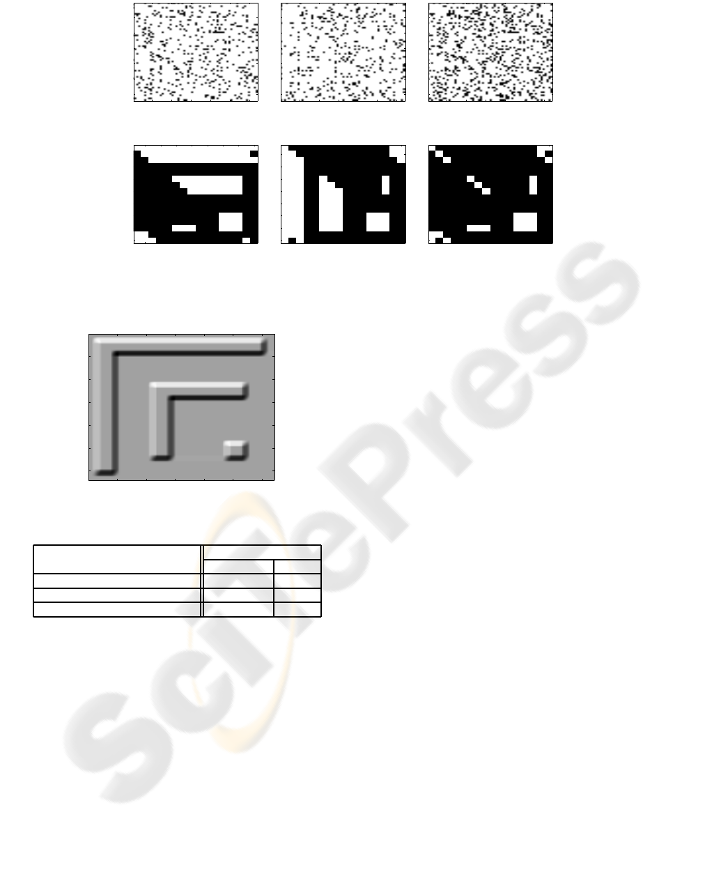
put image is contaminated by additiveGaussian noise.

The advantage of using DHT from noise robustness

standpoint becomes obvious when one observes the

reconstruction using the binarized DHT of the noisy

input image displayed on Figure 11. Here we apply

Gaussian noise with mean = 0 and variance = 0.01.

One can see that in the presence of additive white

noise, no comprehensible information will be con-

tained at the ﬁnest level of the pyramid, see Figure 11

, V

and D

. On the other hand the information is

still available from the level corresponding to s = 3,

i.e. Figure 11 H

, V

and D

. Subsequently, the initial

estimation and the following minimization will not be

badly affected by the noise. The image of the sur-

face reconstructed from the noisy data is displayed on

Figure 12. Finally, error comparison between model

based and variational methods is given on Figure 13.

20 40 60 80 100 120

100

120

Figure 10: Lambertian image of the surface reconstructed

using variational approach from noise free image.

10 20 30 40 50 60

2 4 6 8 10 12 14 16

Figure 11: Binarization of the DHT of the noisy image.

20 40 60 80 100 120

100

120

Figure 12: Image of the surface reconstructed from noisy

data by our method.

Errors, STD

Method, Data type Brightness Depth

Our method, noise free 0.45 0.06

Our method, noisy 0.54 0.48

Variational method, noise free 2.73 2.12

Figure 13: Error comparison.

ACKNOWLEDGEMENTS

The generous support of Applied Materials Inc. is

thankfully acknowledged.

REFERENCES

A. Jones, G. T. (1994). Robust shape from shading. In

Image and Vision Computing, vol 12, no. 7. pp 411-

421.

Atick, J., Grifﬁn, P., and Redlich, A. (1996). Statistical ap-

proach to shape from shading, reconstruction of three-

dimensional face surface from single two-dimensional

images. In Neural Computation 8, pp 1321-1340.

Gill, P., Murray, W., and Wright, M. (1982). Practical Op-

timization. Academic Press, London.

Horn, B. (1975). Obtaining shape from shading informa-

tion. In Psychology of Computer Vision. pp 115-155.

Horn, B. and Brooks., M. (1986). The variational approach

to shape from shading. In Computer Vision, Graphics

and Image Processing, vol 33, no. 1. pp 174-208.

Mallat, S. (1999). A Wavelet Tour of Signal Processing.

Academic Press, London, 2nd edition.

Prados, E., Faugeras, O., and Camilli, F. (2004). Shape from

shading: a well-posed problem ?. In INRIA, Tech. Re-

port. RR-5297.

R. Kimmel, K. Siddiqi, B. K. and Bruckstein., A. M. (1995).

Shape from shading: Level set propagatioin and vis-

cosity solutions. In International Journal of Computer

Vision, vol 16, no. 1. pp 107-133.

Reimer, L. (1993). Image Formation in Low-Voltage Scan-

ning Electron Microscopy. SPIE Press, Bellingham,

USA.

Shapiro., J. (1986). Embedding image coding using ze-

rotrees of wavelet coefﬁcients. In IEEE Trans. on Sig-

nal Processing, vol 41, no. 12. pp 3445-3462.

T. Pong, R. H. and Shapiro., L. (1989). Shape from shading

using the facet model. In Pattern Recognition, vol 22,

no. 6. pp 683-695.

Zhang, R., Tsai, P., Cryer, J., and Shah., M. (1999). Shape

from shading: A survey. In IEEE Trans. PAMI Vol.21,

No. 8 pp 690-706.

Zheng, Q. and Chellappa, R. (1991). Estimation of illu-

minant direction, albedo and shape from shading. In

IEEE Trans. on PAMI, vol. 13, no. 7, pp 680-7021.