
SIMULATION METHODOLOGIES FOR
SCIENTIFIC COMPUTING
Modern Application Design
Philipp Schwaha, Markus Schwaha, Ren
´
e Heinzl
Enzo Ungersboeck and Siegfried Selberherr
Institute for Microelectronics, TU Wien, Gusshausstrasse 27-29, Vienna, Austria
Keywords:
Simulation methodology, Boltzmann transport equation, scientific computing, high performance computing,
programming paradigms, probabilistic method, partial differential equations.
Abstract:
We discuss methodologies to obtain solutions to complex mathematical problems derived from physical mod-
els. We present an approach based on series expansion, using discretization and averaging, and a stochastic
approach. Various forms based on the Boltzmann equation are used as model problems. Each of the method-
ologies comes with its own strengths and weaknesses, which are briefly outlined. We also provide short
code snippets to demonstrate implementations of key parts, that make use of our generic scientific simulation
environment, which combines high expressiveness with high runtime performance.
1 INTRODUCTION
The different natures and complexities of various
equations used to model physical phenomena has
spawned a wide variety of different solution method-
ologies. The corresponding solution techniques usu-
ally exhibit unique characteristics and cover different
aspects of the total solution space.
The methodologies evolved due to the great diver-
sity of needs encountered in application and theory
with the highly relevant goal to cope with the limita-
tions of available computing resources.
The continuous introduction of newer, more so-
phisticated models encourages the use of different
methodologies to best probe the behavior of these new
models. It should also not be underestimated, that
for all the mathematical elegance which many of the
new models may posses, the implementation is often
very tedious due to limitations caused by the notation
available in programming languages. Furthermore,
the constant influx of complexity prohibits any squan-
dering of computational resources, because the added
complexity easily outgrows the evolution of compu-
tational power. It is therefore of utmost importance to
provide resource aware means to realize as many of
the different approaches to solve a given problem as
efficiently as possible.
In answer to this need for an advanced simulation
environment, offering high performance as well as
high expressiveness, we have developed the generic
scientific simulation environment (GSSE), which is a
implements concepts suitable for scientific comput-
ing offers facilities to implement the various simula-
tion methodologies and guaranties high performance
(Heinzl et al., 2006a). Furthermore, it provides great
freedom in the choice of dimension and topology.
This is accomplished by combining several program-
ming paradigms.
In the following we review several established
simulation methodologies and discuss their different
characteristics using examples based on the Boltz-
mann equation, which can easily be transferred to
other fields of research. In the following we distin-
guish the following simulation methodologies:
• Series expansion schemes: choose an analytic
base to parametrize the solution space.
• Discretization schemes: project the original, still
continuous problem into a finite space of algebraic
equations.
• Stochastic schemes: generate local statements
which use statistics to create traces in the solution
space.
We show that a varying interest in the level of detail
270
Schwaha P., Schwaha M., Heinzl R., Ungersboeck E. and Selberherr S. (2007).
SIMULATION METHODOLOGIES FOR SCIENTIFIC COMPUTING - Modern Application Design.
In Proceedings of the Second Inter national Conference on Software and Data Technologies - SE, pages 270-276
DOI: 10.5220/0001338802700276
Copyright
c
SciTePress
of the solution and the amount of affordable compu-
tational resources are best met by different simulation
methodologies.
2 THE GENERIC SCIENTIFIC
SIMULATION ENVIRONMENT
Our approach of transforming different methodolo-
gies into high performance applications is based on
the GSSE. It provides a domain specific embedded
language for mathematical notation as well as data
structures directly within C++, which greatly eases
the specification of formulae and provides the func-
tional dependencies inherent in the formulae.
Another important part of the environment is to
offer consistent interfaces by using concept based
generic programming to achieve interoperability be-
tween different library approaches. Furthermore, we
developed a consistent data structure interface for
all different types of data structures (STL (Austern,
1998), BGL (Siek et al., 2002), GrAL (Berti, 2002),
CGAL (Fabri, 2001)) based on algebraic topology
and poset theory (Heinzl et al., 2006b). With this in-
terface specification we can make use of several al-
ready available libraries within the GSSE. High in-
teroperability and code reuse can thereby be accom-
plished without incurring overhead.
Algebraic topology is used for the interface
and traversal specification further separating the cell
topology from the complex topology. Code complex-
ity is thereby reduced greatly, while at the same time
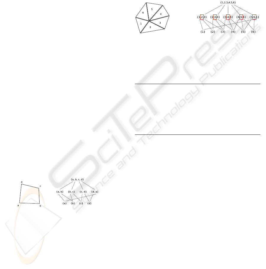
code reuse is increased. Figure 1 depicts the topolog-
ical properties of a cuboid cell and the correspond-
ing projection into a partially ordered set (poset).
Figure 1: Cell topology of a cuboid cell in two dimensions.
Using this poset it is possible to identify all inter-
dimensional objects such as edges and facets and their
relations to the cell. Therefore, traversal of all of
these different objects is completely determined by
this structure and the vertex on edge, vertex on cell,
and edge on cell traversal up to the dimension of the
cell can be derived automatically by the compiler it-
self without the need of user intervention.
In addition to the cell topology the complex topol-
ogy can be derived in order to best support a unique
characterization and orthogonal implementation. A
basic example is depicted in Figure 2, which presents
the structure of a three-dimensional cell complex.
Only locally neighboring cells can be traversed by this
data structure, which can be seen in the poset on the
right hand side. The number of elements in the meta-
cell’s subsets is bounded by a constant number, which
is unique for each type of data structure. The term
meta-cell is used to describe various subsets with a
common name, e.g., the singly linked list uses two
elements per meta-cell, later stated as
local(2)
and
called
forward
concept in the STL.
Figure 2: Complex topology of a three-dimensional simplex
cell complex.
In order to demonstrate the equivalence of our data
structure and the STL data structures a simple code
snippet is presented. The corresponding and required
typedef
definitions are omitted:
cell_type <0, simplex> cells_t;
complex_type <cells_t, global > complex_t;
long
data_t;
container_t <complex_t ,data_t > container;
// is equivalent to the STL type
std::vector<data_t> container;
Equivalence of Data Structures
The distinct areas of scientific computing yield
themselves differently well to implementations us-
ing one of the many programming techniques. In
several cases the demand for a specific program-
ming paradigm can be observed. We provide a short
overview of several programming paradigms and their
advantages:
• Object-oriented programming: is the close inter-
action of content and mechanisms related to the
particular content. Algorithms can not be speci-
fied independently of object structures.
• Functional programming: is inherently parallel
and side-effect free. However, most functional
programming languages suffer from great perfor-
mance shortcomings.
• Generic programming: is the glue between object-
oriented programming and functional program-
ming.
Many difficulties encountered in conventional pro-
gramming can be circumvented with the approach
of using the paradigms shown above appropriately
at the same time. Functional programming enables
SIMULATION METHODOLOGIES FOR SCIENTIFIC COMPUTING - Modern Application Design
271

great extensibility due to the modularity of func-
tion objects. Generic programming and the corre-
sponding template mechanisms of C++ offer high per-
formance combined with parametric polymorphism.
This means that arbitrary data structures of arbitrary
dimensions can be used.
GSSE has been implemented making strong use
of the generic programming to reduce the amount of
code which has to be maintained. The realization
of the generic programming facilities in C++ as tem-
plates ensures high run time performance, as the com-
piler is free to generate the most appropriate code.
As the focus of this paper is the comparison of dif-
ferent simulation methodologies, performance details
(Heinzl et al., 2006a) have to be omitted due to space
constraints. As already pointed out the interfaces of
GSSE are compatible to the STL, which facilitates
code re-usability enormously.
3 BOLTZMANN’S EQUATION
From the many different equations used to describe
our physical reality, Boltzmann’s equation has shown
to be one of the most versatile. Originally conceived
to govern the dynamics of particles in gases and flu-
ids, it is for instance also used to describe the dis-
tribution of electrons in semiconductors. Due to the
complexity inherent to Boltzmann’s equation several
solution techniques have been developed. The meso-
scopic nature of Boltzmann’s equation makes it also
well suited for the development of simpler models,
such as the drift-diffusion model.
Boltzmann’s equation for electron transport in
semiconductors, as given in Equation 1, is the base for
many calculations regarding microelectronics (Sel-
berherr, 1984).
∂
∂t
f +~v· grad
r
f +
~
F · grad
p
f =
∂
∂t
f|
collisions
(1)
Here f is the distribution function which depends on
the location (r) as well as the momentum (p). ~v is
the velocity of the electrons, while
~
F denotes a force
acting on the electrons. The right hand side of Equa-
tion 1 describes the changes of the distribution func-
tion due to collisions. Macroscopic quantities such
as the concentrations of the electrons can then be cal-
culated from the distribution function by integration,
such as
n =
fd
3
p
The term~v· grad
r
f describes the displacement of the
distribution due to the velocity of the electrons. The
velocity is obtained from the electron’s dispersion re-
lation ε(~p) as
~v = grad
p
ε(~p) (2)
thereby linking the dispersion relation explicitly to the
distribution function.
The term
~
F ·grad
p
f links an external force
~
F act-
ing on the electrons to their distribution. It can be ex-
pressed as
~
F = q
~
E with q being the elementary charge
and
~
E being the electric field.
The term describing the collisions is often mod-
eled in the form of
∂
∂t
f|
collision
=
V
(2π)
3
f(~x,~p
′
)S(~p
′
,~p) d
3
~p
′
−
V
(2π)
3
f(~x,~p)S(
~
k,~p
′
) d
3
~p
′
(3)
Where the terms S(~p,~p
′
) is the transitions from one
momentum state ~p to another ~p
′
. The various phys-
ical scattering mechanisms are modeled by adjusting
these terms appropriately (Kosina, 2003).
4 METHODOLOGIES
Having introduced our framework and the basic equa-
tion under consideration we now present three dif-
ferent methodologies. Each of the methodologies
has a different characteristic of the obtained solution
and emphasizes different aspects of the computations.
The choice of an appropriate methodology depends
highly on the requirements placed on the obtained
solution and its cost in terms of time and computa-
tional expense. It is therefore necessary to have an, at
least basic, understanding of what a given methodol-
ogy can accomplish.
4.1 Series Expansion Schemes
Unfortunately differential equations for which elegant
solutions using closed form analytical functions exist,
are a rare special case for models of physical phenom-
ena.
The notion of obtaining a solution or at least an ad-
equate approximation by analytical means, however,
is highly attractive. In order to utilize this approach,
it is necessary to thoroughly analyze the problem for
exploitable properties, such as symmetries, and make
use of them.
The old idea of series expansion provides the
means to accomplish this goal. Here the function is
represented as a sum of several terms:
f =
b
∑
i=a
c
i
β
i
The c
i
are the coefficients for the base β
i
of the ex-
pansion. Summation takes place for a− b values. In
ICSOFT 2007 - International Conference on Software and Data Technologies
272

theory a and/or b may be infinite to obtain an exact
solution.
Since it is obviously not possible to evaluate an
infinite number of summations, the series has to be
truncated. An appropriate choice of β determines the
accuracy of this solution method, when truncating the
series at a given order. The better β is able to reflect
the properties of the true solution, the more accurate
the truncated solution becomes.
We now apply the method of series expansion
to Boltzmann’s equation using spherical harmonics
(Abramowitz and Stegun, 1964) for expansion. The
spherical harmonics used are defined as:
Y
m
n
(ϑ,ϕ) = (−1)
m
s
2n+ 1
4π
(n− m)!
(n+ m)!
P
m
n
(cosϑ) e
imϕ
With P
m
n
being associated Legendre polynomials.
The leading factor ensures the orthonormality of the
spherical harmonics.
Expanding the distribution functions using spher-
ical harmonics and using the physics governing the
movements of electrons it is possible to obtain the
following equation system for the left hand side of
Boltzmann’s equation:
∞
∑
s=0
s
∑
w=−s
div
r
g
w
s
Y
w
s
~v Y
m
l
dΩ+ ~
~
F
∂
∂ ε
g
w
s
Y
w
s
~v Y
m
l
dΩ
−
~
Fg
w
s
Y
w
s
grad
k
Y
m
l
dΩ
ε is the energy of an electron, ~ is Planck’s re-
duced constant, and the g
w
s
are transformed coeffi-
cients of the expansion. The first line of the equa-
tion is given in the following source snippet, where
the
sum<>(start,end,local variable)
is derived
from the Boost Phoenix 2 (Boost Phoenix 2, 2006)
environment with local scope variables. The integrals
have to be evaluated just once (
pre int<1>
) and are
then constants entered into the equation system. Their
evaluation is made easier due to the orthogonality of
the spherical harmonic basis functions.
linearequ_t equation_gsw;
equation_gsw = (sum<>(0,limit ,_s)
[
sum<>(-_s,_s,_w)
[
sum<vertex_edge >
[
g_quan(_s,_w)
] * vol / area * pre_int<1>
]
]) (vertex);
Assembly of the Equation System for the Expansion Coef-
ficients
After the equation system for the coefficients is as-
sembled and solved, the solution to the initial problem
is obtained by evaluating the expansion using the cal-
culated coefficients. This also reveals the problems of
this approach. An equation system has to be solved
in order to obtain the coefficients. Furthermore the
evaluation of the expansion may pose additional nu-
merical challenges (Deuflhard, 1976).
4.2 Discretization Schemes
The lack of computational power required for the rig-
orous solution of Boltzmann’s equation resulted in the
development of simplifications that can be used to cal-
culate several important macroscopic quantities.
One of these simplifications is the drift-diffusion
model, which can be derived from Equation 1 by ap-
plying the method of moments (Selberherr, 1984). By
calculating appropriate statistical averages it is possi-
ble to obtain the electron concentration. It is how-
ever not possible to provide more sophisticated in-
formation such as the energy of the electrons. This
approach has been used very successfully in semi-
conductor simulation for several decades now and is
still very popular, although more rigorous alternatives
have been developed.
Equation 4 shows the resulting equation to be
solved self consistently with Poisson’s equation,
given in Equation 5.
div J
n
= 0, J
n
= qnµ
n
grad Ψ+ qD
n
grad n (4)
div (grad ε Ψ) = −ρ (5)
Equation 4 is discretized using the Scharfetter-
Gummel (Scharfetter and Gummel, 1969) scheme re-
sulting in a non-linear equation of the form
J
n,ij
=
q µ
n
U
th
d
ij
n
j
B(Λ
ij
) − n
i
B(−Λ
ij
)
(6)
Λ
ij
=
Ψ
j
− Ψ
i
U
th
B(x) =
x
e
x
− 1
(7)
The discretization of the differential operators using
finite volumes yields:
div x ≈
∑
v→e
x
A
V
grad x ≈
1
d
∆
e→v
x (8)
The formulation so obtained can be implemented
using virtually any programming language, but high
performance is greatly desirable. In order to make
maintenance of the code as easy as possible and to
achieve a maximum of flexibility it is important to
keep the code expressive. With GSSE we achieve
both of these seemingly contradicting goals at the
same time.
SIMULATION METHODOLOGIES FOR SCIENTIFIC COMPUTING - Modern Application Design
273

linearequ_t equation_pot ,
equation_n;
equation_n = (sum<vertex_edge >
[ diff <edge_vertex >
(-n_quan*Bern(
diff<edge_vertex >[pot_quan / U_th]
),
-n_quan*Bern(
diff<edge_vertex >[-pot_quan / U_th]
)
)* (q * mu_h * U_th)
]) (vertex);
equation_pot = (sum<vertex_edge >
[ diff <edge_vertex > [pot_quan]
] + ( n_quan - p_quan + nA - nD ) *
vol * q / (eps0 * epsr)
) (vertex);
Discretized Drift-Diffusion Equation
The benefits of this approach are the simplification
of the model and a tremendous reduction of required
computing resources. The drawbacks again include
the necessity to solve an equation system and the re-
duced amount of information remaining in the calcu-
lated solution.
4.3 Stochastic Schemes
The Monte Carlo (MC) approach is the most impor-
tant stochastic scheme used to simulate physical and
mathematical systems which can not be solved in
more traditional ways due to their complexity. This
is often the case when simulating fluids or gases, or
when the inputs to the simulation are subject to con-
siderable uncertainty and fluctuation.
The MC approach is based on the use of sequences
of random or pseudo random numbers. To get sta-
tistically relevant results thousand if not millions of
variates need to be calculated, which makes MC sim-
ulations computationally very expensive.
Nevertheless, the complexity of the model is bro-
ken down, as the governing equations are evaluated
only locally for each particle and the particle is traced
as it moves through the simulation domain. MC sim-
ulation does not involve the solution of any large sys-
tem of equations to yield a result. As a consequence
ill posed problems are less of a problem and the af-
fordable simulation time becomes the main limiting
factor for this method.
4.3.1 Application Design
We have extracted the most important parts of a MC
application and developed several generic modules:
• Generic random number library interface
• Geometric operations
• Traversal mechanisms
One of the most important parts of the MC simula-
tion is the handling of the random number generator.
We therefore use a generic random number library in-
terface to keep the implementation details and num-
ber distribution orthogonal to the main application.
The current implementation uses the Boost random
number library (Boost, 2007) with overall high per-
formance.
All geometrical operations, such as intersection
tests, angle calculation, and trajectory calculation are
used in several separate modules. Due to the concept
interface these modules can be implemented, e.g.,
with CGAL algorithms (Fabri, 2001) as well. The
CGAL offers additional mechanism of several nu-
merical kernels (Pion and Fabri, 2006) with different
types of accuracy and runtime requirement. An ex-
ample of the main control module for a dimensionally
independent application is presented in the next code
snippet:
template
<
typename
RNG>
void
particle_sim(gsse::domain_t domain ,
std::vector<particle_t >& particles ,
long
iterations , RNG& random_gen) {
for
(
long
j = 0; j < iterations; j++) {
for
(
unsigned int
i = 0;
i < particles.size(); i++) {
// control condition
if
(particles[i].E != 0) {
MC_step(domain ,
particles[i],
random_gen()); }
}
}
}
Control Unit for a Monte Carlo Application
A typical example of an implementation of a MC
application is given next. Different properties can be
written on all cells and the corresponding sub-cells,
such as the reflecting property to an edge.
void
MC_step(gsse::domain_t domain,
particle_t& par,
double
random)
{ std::vector<facet_type > border_facets;
bool
status;
new_position = par.position +
par.delta_t * par.v_vec;
status = particle_in_domain(domain,
new_position);
// evaluate status .. code omitted
do
{ border_facet_intersection(domain,
par, new_position , random);
ICSOFT 2007 - International Conference on Software and Data Technologies
274
par.position = intersection_point;
}
while
(par.E != 0.0);
}
Step Control for a Monte Carlo Application
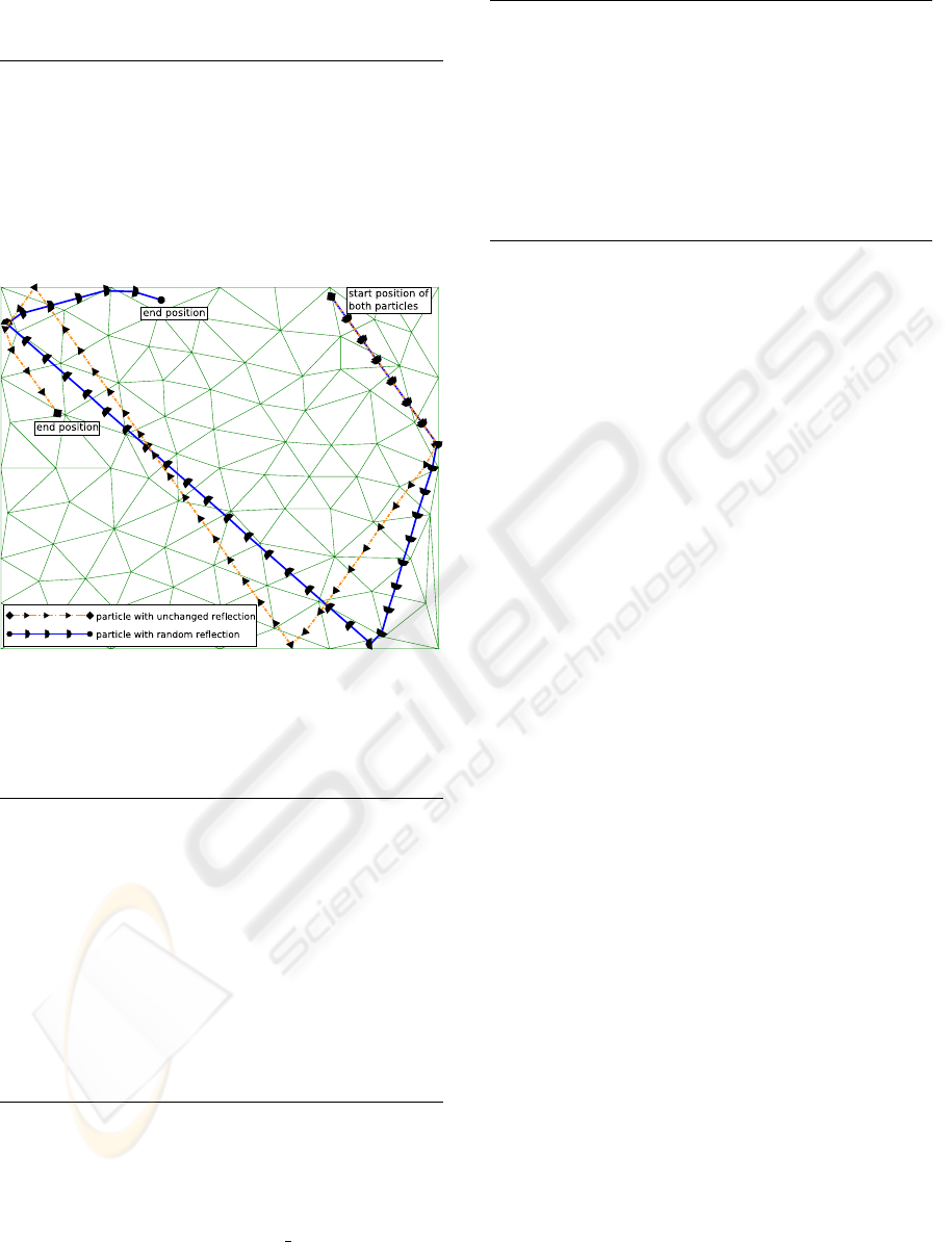
By providing an ability to specify the reflection prop-
erties it is possible to realize the exact as well es dif-
fuse reflections. Figure 3 shows how a single particle
may take different paths, while each reflection is se-
lected randomly, parametrized according to values on
the boundary edges to achieve the effects of diffuse
reflection.
Figure 3: Comparison of trajectories of a particle with ran-
domized and non randomized reflection.
The dimensionally independent implementation
of a geometric test for an intersection with a boundary
is just as simple:
bool
part_in_domain(domain_t domain ,
point_type point)
{
bool
status =
false
; // particle
for
(boundary_cell_iterator
bcit = domain.bcell_begin();
bcit != domain.bcell_end(); ++cit)
{
// geometrical intersection tests for
// a given point with boundary cells
}
return
status;
}
Test for Boundary Intersection
The following code example presents a generic
intersection test of a point and a line. With the
topological interface of the GSSE the CGAL data
structures can be used for all parts of the simulation,
in this example a
CGAL::Segment 2
.
CGAL::Segment_2 <Kernel> domain_t;
CGAL::Line_2 <Kernel > line_t;
void
geom_intersection(domain_t domain,
line_t line, point_type ipoint)
{
CGAL::Object result;
CGAL::Segment_2 <Kernel> iseg;
result=CGAL::intersection(seg, line);
// evaluate the result..
}
Test if a Point Intersects a Line
5 CONCLUSION
We have presented three different methodologies of
obtaining a solution to mathematical equations which
model physical problems. While the availability of
flexible high performance environments greatly eases
application development, each of the different ap-
proaches has its benefits and its drawbacks to be con-
sidered carefully before choosing the implementa-
tion of a solution strategy. Our multi-methodology
environment GSSE eases comparison and develop-
ment greatly by providing all not only all the required
traversal mechanism, thereby eliminating error prone
index operations, but also a functional calculus, that
allows for a mathematically attractive formulation.
REFERENCES
Abramowitz, M. and Stegun, I. A. (1964). Handbook of
Mathematical Functions with Formulas, Graphs, and
Mathematical Tables. Dover, New York.
Austern, M. H. (1998). Generic Programming and the
STL: Using and Extending the C++ Standard Tem-
plate Library. Addison-Wesley Longman Publishing
Co., Inc., Boston, MA, USA.
Berti, G. (2002). GrAL - The Grid Algorithms Library. In
ICCS ’02: Proc. of the Conf. on Comp. Sci., volume
2331, pages 745–754, London, UK. Springer-Verlag.
Boost (2007). Boost C++ Libraries 1.33.
http://www.boost.org.
Boost Phoenix 2 (2006). Boost Phoenix 2.
http://spirit.sourceforge.net/.
Deuflhard, P. (1976). Algorithms for the Summation of Cer-
tain Special Functions. Journal Computing, 17(1):37–
48.
Fabri, A. (2001). CGAL - The Computational Geometry
Algorithm Library.
http://citeseer.ist.psu.edu/fabri01cgal.html.
Heinzl, R. and Schwaha, P. (2007). Generic Scientific Sim-
ulation Environment. http://www.gsse.at.
SIMULATION METHODOLOGIES FOR SCIENTIFIC COMPUTING - Modern Application Design
275

Heinzl, R., Schwaha, P., Spevak, M., and Grasser, T.
(2006a). Performance Aspects of a DSEL for Scien-
tific Computing with C++. In Proc. of the POOSC
Conf., pages 37–41, Nantes, France.
Heinzl, R., Spevak, M., Schwaha, P., and Selberherr, S.
(2006b). A Generic Topology Library. In Library
Centric Sofware Design, OOPSLA, pages 85–93, Port-
land, OR, USA.
Kosina, H. (2003). VMC: a Code for Monte Carlo Sim-
ulation of Quantum Transport. In Proc. 12th MEL-
ARI/NID Workshop.
Pion, S. and Fabri, A. (2006). A Generic Lazy Evaluation
Scheme for Exact Geometric Computations. In Li-
brary Centric Sofware Design, OOPSLA, pages 75–
84, Portland, OR, USA.
Scharfetter, D. and Gummel, H. (1969). Large-Signal Anal-
ysis of a Silicon Read Diode Oscillator. IEEE Trans.
Electron Dev., 16(1):64–77.
Selberherr, S. (1984). Analysis and Simulation of Semicon-
ductor Devices. Springer, Wien–New York.
Siek, J., Lee, L.-Q., and Lumsdaine, A. (2002). The Boost
Graph Library: User Guide and Reference Manual.
Addison-Wesley.
ICSOFT 2007 - International Conference on Software and Data Technologies
276
