
A MULTIDIMENSIONAL APPROACH TO THE
REPRESENTATION OF THE SPATIO-TEMPORAL
MULTI-GRANULARITY
Concepción M. Gascueña, Dolores Cuadra, Paloma Martínez
Computer Science Department University Carlos III Madrid, Avenida de la Universidad 30 Leganés 28911 Spain
Keywords: Multidimensional model, Spatio-temporal Database, Spatio-temporal multi-granularity representation,
Spatial Datawarehouse.
Abstract: Many efforts have been made to the treatment of spatial data in databases both in traditional database
systems and decision of support systems or On-Line Analytical Processing (OLAP) technologies in
datawarehouses (DW). Nevertheless, many open questions concerning this kind of data still remain. The
work presented in this paper is focused on dealing with the spatial and temporal granularity within a logical
multidimensional model. We propose an extension of the Snowflake model to gather the spatial data and to
show our proposal to represent the spatial evolution through time in a simple and intuitive way. We
represent the temporal and spatial multi-granularity with different levels in the hierarchies of dimensions,
and we present a typology of hierarchies to include more semantics in the Snowflake scheme.
1 INTRODUCTION
Many works have addressed the study of the
treatment of spatial data and its management in
Database to avoid inconsistencies caused by
Geographic Information Systems (GISs), which
make a heterogeneous treatment of data separating
spatial data and storing them in file systems and
non-spatial data, in general, stored in database
systems. Nevertheless, these are still many questions
unresolved when managing this singular data. One
of these questions is derived from the use of spatial-
temporal data and is related to the granularity
definition. The spatial granularity is defined as the
unit of measure chosen to represent the spatial
element within a given reference system. The
temporal granularity is defined to represent the
variations of an element, through time. The spatial-
temporal multi-granularity represents the units of
measurement chosen to store a geometric object in
different moments of time. Many studies measure
time in intervals, but in our proposal we will use
points in time which, due to their simplicity, avoid
the problem of coalescence. The main objective of
this proposal is to enrich the Multidimensional
models from a logical point of view to include
semantics and information about spatio-temporal
data. We propose an extension of the Snowflake
scheme to gather both the spatial granularity and the
temporal granularity. This paper is organized as
follows: Section 2 contains references to works
related to the treatment of the spatial and temporal
data in databases. Section 3 contains logical
multidimensional concepts. Section 4 is made a
proposal for the multi-granular treatment using the
Snowflake scheme. Section 5 presents several
examples to clarify our proposal and some
conclusions are given in section 6.
2 RELATED WORKS
There is a great amount of research about the special
characteristics of the spatial data and its
representation in Multidimensional schemes.
(Sefanovic et al., 2000) distinguish between three
types of spatial dimensions, according to whether
the spatial elements are include in every hierarchy,
in some hierarchy or in no hierarchy. Also they
consider two types of measures, spatial and
numerical. (Miquel et al.,2004) establish that if a
spatial measure is required in the fact table, then the
model must include a spatial dimension, as opposed
175
M. Gascueña C., Cuadra D. and Martínez P. (2006).
A MULTIDIMENSIONAL APPROACH TO THE REPRESENTATION OF THE SPATIO-TEMPORAL MULTI-GRANULARITY.
In Proceedings of the Eighth International Conference on Enterprise Information Systems - DISI, pages 175-180
DOI: 10.5220/0002495801750180
Copyright
c
SciTePress
to (Malinowski and Zimanyi , 2004) who propose
the inclusion of the spatial data in the different
levels of a hierarchy and also in measures. (Rives et
al., 2001), study the spatial data in the dimensions
and in the fact table. (Kouba et al. 2002) treat the
navigation consistency among the levels of the
hierarchies for spatial data and OLAP systems. (Han
et al., 1997), establish Spatial On-Line Analytical
Processing (SOLAP) prototypes that gather the
concepts of OLAP and apply them to spatial data.
The proposal of (Pourabbas et al.) and (Ferri et al.,
2000) integrates GIS systems and DW/OLAP
environments. None of these approaches define the
spatio-temporal multi-granularity concept.
According to (Camossi, et al.,2003) the spatio-
temporal multi-granularity concept is very important
in representing the semantic of domain.
3 MULTIDIMENSIONAL
CONCEPTS
A Data Warehouse (DW) is defined as a collection
of subject-oriented, integrated, non-volatile data that
vary in time, which support decision making
processes (Sefanovic et al., 2000). DW are usually
represented at a logical level by multidimensional
models and these use Star, Snowflake or the
Constellation scheme. A logical multidimensional
model consists of different elements: dimensions,
hierarchies and fact tables. A fact table contains the
focus of analysis and subject-orientation, e.g.
analysis of daily sales of stores in a city. Also a fact
table contains measures, based on the dimensions,
that reflect a characteristic whose evolution we wish
obtain. In the previous example, the sales are
measures and the stores, the city, and the days are
dimensions. The Dimensions provide a view of the
data from different perspectives and the hierarchies
provide a more generalized view of them. The
dimensions can form hierarchies like Day-Month-
Year and moreover, they can contain attributes that
complete information, such as holidays in a month.
The Star scheme consists of dimensions, without
hierarchies, and a fact table with measures. The
Snowflake scheme permits that the attributes of
dimensions are structured into different groups.
These groups form levels and these levels form a
hierarchy. The Constellation scheme can contain
several fact tables in the scheme, each one with its
corresponding measures and these fact tables can
share it’s hierarchies. Within a hierarchy, the lower
level is called leaf level. The OLAP Systems allow
dynamic manipulation of the DW for the process of
decision making. The SDWs combine DW and
Spatial System Databases and allow storage of huge
volumes of spatial data, spatial statistical analysis
and spatial data mining. We use an extension of the
Snowflake scheme to include spatial data and make
our proposal.
4 INCLUDING
MULTI-GRANULARITY IN A
SNOWFLAKE SCHEMA
We propose a extension of the Snowflake scheme
due to its intuitive manner of representing the
evolution of an object through time. The aim is to
add semantic information to the scheme. We
propose to treat the spatial and temporal granularity
as dimensions in the Snowflake schema.
Table 1: Temporal conversion functions.
It returns, for each granule in the coarser granularity, the value which
always appears in the included granules at the finer granularity if this
value exists, the null value otherwise
All
It returns, for each granule in the coarser granularity, the value which
appears most frequently in the included granules at the finer granularity
Main
First and last index in the Proj (index) function
First,, Last
It returns, for each granule in the coarser granularity, the value corresponding
to the granule of position index at the finer granularity
Proj (index)
It returns, for each granule in the coarser granularity, the value which
always appears in the included granules at the finer granularity if this
value exists, the null value otherwise
All
It returns, for each granule in the coarser granularity, the value which
appears most frequently in the included granules at the finer granularity
Main
First and last index in the Proj (index) function
First,, Last
It returns, for each granule in the coarser granularity, the value corresponding
to the granule of position index at the finer granularity
Proj (index)
In order to operate and compare objects with
different granularity, we must use conversion
functions. Some conversion functions are shown in
Table 1 and Table 2. The application of these
functions guarantees the topology consistency
(Camossi et al., 2003).
Table 2: Patial conversion functions.
It contracts an open line, endpoints included, to a pointl_contr
It contracts a simple connect region and its bounding to a pointr_contr
It eliminates (abstracts) an isolated point inside a regionP_abs
Absorption operations
It eliminates a line inside a regionl_abs
It merges two regions sharing a boundary line into a single regionr_merge
It merges two lines sharing an endpoint into to single linel_merge
Merge functions
It reduces a region and its bounding lines to a liner_thinning
Contract functions
Table 2.1: Some conversion functions for
multidimensional model.
M_Last
Mr_thinning
Mr_contr
Ml_contr
It chooses the last element within a rank
It reduces a region and its bounding lines to a line
It contracts a simple connect region and its bounding to a point
It contracts an open line, endpoints included, to a point
M_Last
Mr_thinning
Mr_contr
Ml_contr
It chooses the last element within a rank
It reduces a region and its bounding lines to a line
It contracts a simple connect region and its bounding to a point
It contracts an open line, endpoints included, to a point
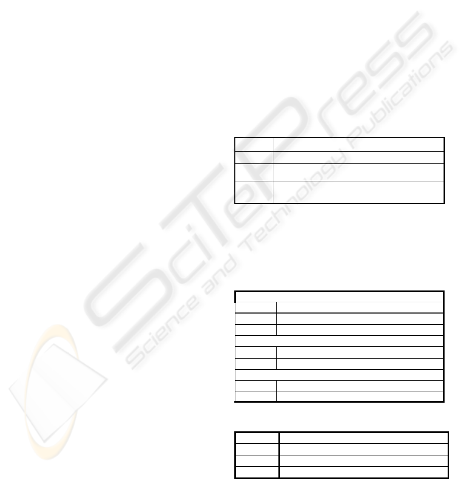
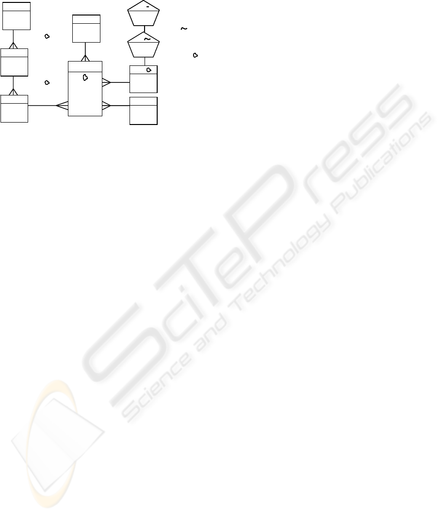
We propose a notation based on multidimensional
concepts (see Figure1).
ICEIS 2006 - DATABASES AND INFORMATION SYSTEMS INTEGRATION
176
In order to represent the different spatial
granularities, we propose to include a new type of
hierarchy called Static hierarchy. This hierarchy
type is different from the ones used previously by
the multidimensional scheme. Each spatial
granularity will be treated as a level within this
hierarchy.
The Dynamic hierarchy, (figure 1,h), where the
route (navigate) from one level to another implies
changes in measures of the fact table. The Static
hierarchy, (figure 1,i), where the route (navigate)
from one level to another does not imply changes in
measures of the fact tables. Nevertheless, Static
hierarchies contribute semantically to the model and
provide clarity in the study of facts in the decision
making processes.
Each Static hierarchy level, different to leaf level, is
graphically represented by a pentagon (figure 1,o).
We define the granularity within hierarchy as
follows: a granularity g
1
is finer_than another one
g
2
, if g
1
∈N
1
and g
2
∈N
2
where N
1
< N
2
and N
1
,N
2
∈J
i
and J
i
∈D
k
where N
1
and N
2
are levels of the
hierarchy J
i
. Where J
i
is a hierarchy of the D
k
dimension and also g1 ⊆ g2.
Topological RelationshipaSapatial Data Type
Cros Point and LinePoint
Cross Line and LineLine
Cross Surface and LineSurface
Topological RelationshipaSapatial Data Type
Cros Point and LinePoint
Cross Line and LineLine
Cross Surface and LineSurface
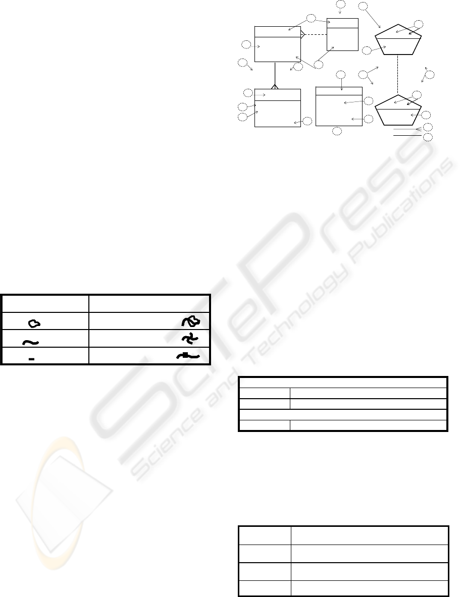
Figure 2a: Some spatial data types and topological
relationships.
The leaf level marks the finer granularity in each
dimension. In order to navegate between different
levels of hierarchies, we use multidimensional
operators, some of these are shown in (Figure 2,b).
To represent the geometry of the spatial data, we use
SQL3 with its extension to spatial data type and the
topological relationships among them, according to
OpenGis Specification (Figura 2,a). In order to show
the conversion function that we wished for when
applying Roll-up in the hierarchy, we introduced a
new label in the scheme. (Figure 1,j) (Figure 1,k).
We think that it is important to express the
aggregation functions used when we navigate
through different levels of hierarchies. Some
funtions are shown in Table3 and Table4.
Leaf Level
Key attibute
Aggregate Function (Measure1)
Key attribute
Secondary attribute
------
Level 1
Key attibute
Dimension with a Dimension with a
Dinamic Hierarchy S tatic Hierarchy
Transformation Function 1(Spatial Measure)
c
a
d
c
e
f
h
j
b
k
o
i
j k
Granularity n Geometry n
Granularity 1 Geometry 1
m
n
o
Transformation Function n(Spatial Measure)
Fact Table
Measure 1
…..
Measure n
Key Dimension 1
-------------
Key Dimension n
Level n
g.1
g.2
g.3
l
l
g
Leaf Level
Key attibute
Aggregate Function (Measure1)
Key attribute
Secondary attribute
------
Level 1
Key attibute
Dimension with a Dimension with a
Dinamic Hierarchy S tatic Hierarchy
Transformation Function 1(Spatial Measure)
c
a
d
c
e
f
h
j
b
k
o
i
j k
Granularity n Geometry nGranularity n Geometry nGranularity n Geometry n
Granularity 1 Geometry 1Granularity 1 Geometry 1Granularity 1 Geometry 1
m
n
o
Transformation Function n(Spatial Measure)
Fact Table
Measure 1
…..
Measure n
Key Dimension 1
-------------
Key Dimension n
Fact Table
Measure 1
…..
Measure n
Key Dimension 1
-------------
Key Dimension n
Fact Table
Measure 1
…..
Measure n
Key Dimension 1
-------------
Key Dimension n
Level n
g.1
g.2
g.3
l
l
g
a) Dimension table of leaf level
b) Dimension table of a dynamic hierarchy
c) Key attributes as primary key of each level
d) Secondary Attributes that complete information of
each level
e) Name of the leaf level
f) Name of level
g)
Fact table: g.1 Fact table name, g.2 Measure, focus
of analysis, g.3 Key from dimensions.
h) Dynamic Hierarchy
i) Static Hierarchy
j) Label expressing the associate function from each
measure in roll-up of dimensions
k) Measure in which function is applied
l) Representation of geometry and units expressed in a
spatial reference
m) The cardinality 1:N, between levels
n) The cardinality 1:1, between levels
o) Represents a level in a static hierarchy
Figure 1: Notation for a Logical Model.
Selection and projection of elementsSlice, Dice
Selecting elements
Navigating from higher level to lower levelDrill-Dow
Navigating from lower level to higher levelRoll-up
Navigating through the levels of hierarchy
Selection and projection of elementsSlice, Dice
Selecting elements
Navigating from higher level to lower levelDrill-Dow
Navigating from lower level to higher levelRoll-up
Navigating through the levels of hierarchy
Figure 2b: Multidimensional Operators.
We distinguish between thematic dimension
which do not contain spatial data and spatial
dimension that contain spatial data.
Table 3: Non Spatial data Functions.
User Defined
Median, most frequent, rank.. Required new calculations using
the data of the leaf level
Holistic
Average, Variance, Standard deviation,…. Need an additional
treatment for reusing the values
Algebraic
Sum, Min, Max…Reuse aggregates of a lower level of a
hierarchy in order to calculate the aggregates for higher level
Distributive
We present our proposal studing the spatial data
within the fact table according to if it is treated as a
measure or as a dimension with some examples: In
A MULTIDIMENSIONAL APPROACH TO THE REPRESENTATION OF THE SPATIO-TEMPORAL
MULTI-GRANULARITY
177
the example 1, we study when spatial data is only
one spatial dimension present in the fact table,
(Figure 3).
In the example 2 we study when there is more
than one spatial dimension and in addition, spatial
data acts as measures within the fact table, these
spatial elements must be related among them to
some of spatial topological relations (spatial join)
described in Figure (2 a), (Figure 4).
Table 4: Spatial data Functions.
User Defined
Equi-partition, nearest-neighbor indexHolistic
Center of n geometric points, center of gravityAlgebraic
Convex hull, geometric union, geometric intersectionDistributive
User Defined
Equi-partition, nearest-neighbor indexHolistic
Center of n geometric points, center of gravityAlgebraic
Convex hull, geometric union, geometric intersectionDistributive
In the example 3, the spatial data is a measure within
the fact table and we want to study its evolution in
time from different granulaties, (Figure5).
We used the functions in (Table 2,1) as an
extension of Table 1 and Table 2. For the example,
we define a spatial object as a data type abstract
with an identity, a granularity, a geometry of
representation and a temporal granularity. The
granularity or unit of measure is associated to a
reference system. The geometry of representation is
associated to a dimension. We will utilize
geometries of two dimensions and the metric system
as reference. Although there are many more cases,
the size of this study prevents us from locking at all
of them.
5 JUSTIFYNG WE APPROACH
Example 1. We want to manage the collected
agricultural production of a set of plots through the
time. We wish to store the production as kilograms
of product gathered per semester in each plot. The
Plots have certain geography and we want to store
its area in meters and its changes for semester, as
well as the plot owner identified by the SSN. We
consider that the production of each plot is only one
product that does not vary in time, though the same
product can be simultaneously cultivated in several
plots.
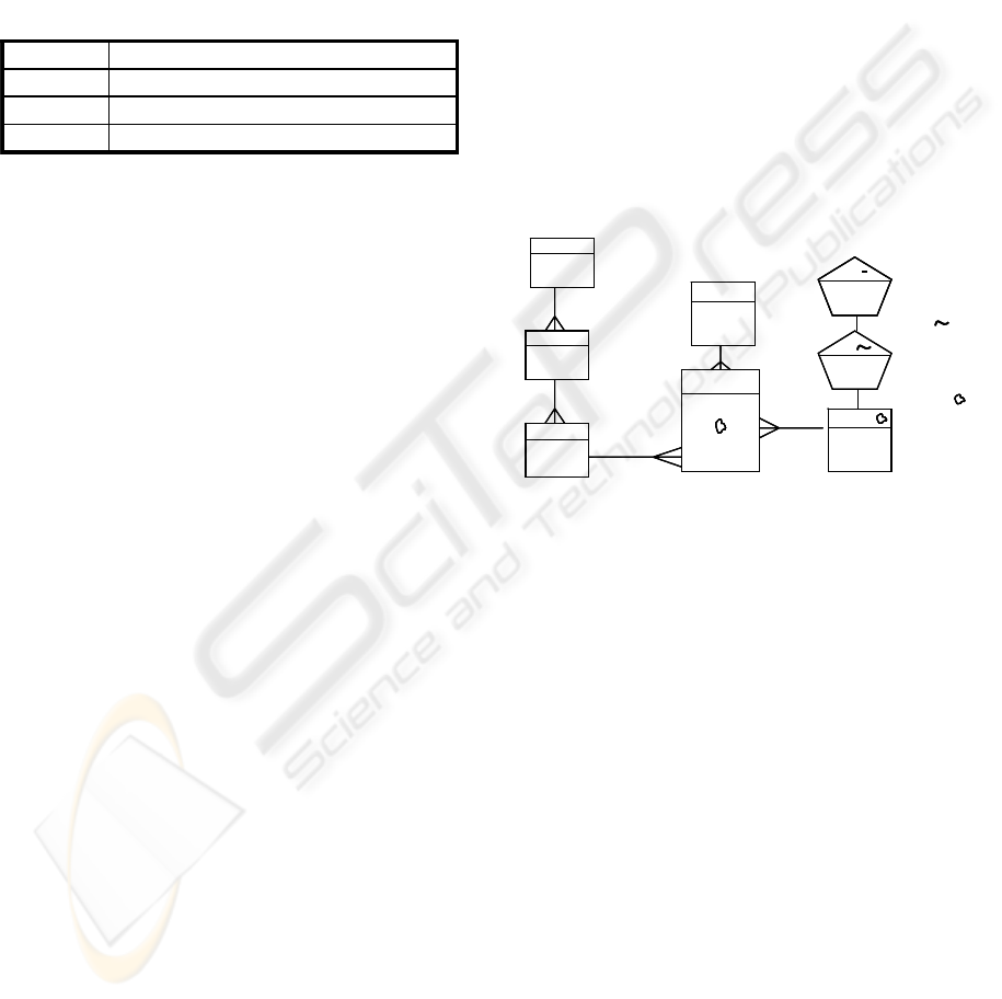
We model this example with the extension of the
Snowflake scheme proposal (Figure 3). We have
three dimensions: Time Dimension, Owner
Dimension, and Plot Space Dimension; and a
Production fact table. The Time dimension is
established with three granularities: semester, year
and decade, and are represented in a hierarchy with
three levels, one for each granularity. Here, the
temporal dimension marks the time of changes of all
the dimensions. In the Plot dimension three
granularities are defined, Meter, Hectometer, and
Kilometer with three levels. The smaller granularity,
leaf level, represents spatial data with a geometry of
surface measured in meters; the second level
represents the spatial data with a lineal geometry
measured in hectometers; and the third level, the
data is represented with a point measured in
kilometers (Figure 2,a). The Owner dimension does
not have spatial data and it does not have any
hierarchy. The Production fact table has one
measure, KProd, which gathers the production of
each plot every semester; it also contains the keys of
leaf level of each dimension; the set of these keys
form the key of this fact table.
Production
KProd
IDP m
Sem_x
SSN
Year
Decade
Semester
Sem_x
Mr_thinning (IDP )
Ml_contr(IDP )
Plot Space Dimension
Static Hierarchy
Time Dimension
Dynamic Hierarchy
Owner Dimension
Hm
Km
Plot m
IDP
Product
Sum (KPro )
Sum (KPro )
Owner
SSN
…..
Production
KProd
IDP m
Sem_x
SSN
KProd
IDP m
Sem_x
SSN
Year
Decade
Semester
Sem_x
Mr_thinning (IDP )
Ml_contr(IDP )
Plot Space Dimension
Static Hierarchy
Time Dimension
Dynamic Hierarchy
Owner Dimension
Hm
KmKmKm
Plot m Plot m Plot m
IDP
Product
Sum (KPro )
Sum (KPro )
Owner
SSN
…..
Owner
SSN
…..
Owner
SSN
…..
Figure 3: Example with one spatial dimension present in
the fact table.
We can see that the key of the Plot dimension is
spatial data, which contains an identity and a
geometry of surface associated with the unit metre.
Also, this key is propagated inside the fact table. As
we want to represent spatial data along with the
measure KProd.
The hierarchy of the Temporal dimension is a
dynamic hierarchy because it implies changes in the
measure of the fact table when navigating through
its levels. When doing Roll-up in the Time
dimension, i.e. we change the temporal granularity
from a smaller granularity to another more coarser
granularity, the aggregation function which we need
apply to Kprod measure the function Sum, the same
as for all levels. The hierarchy of the Plot spatial
dimension is an example of static hierarchy, because
KProd measure does not change when navigating
through its levels, however the spatial granularity of
plot spatial element changes. Thus, when making the
Roll-up from the leaf level to the second level of this
static hierarchy, the Mr_thinning function is applied
ICEIS 2006 - DATABASES AND INFORMATION SYSTEMS INTEGRATION
178
(Table 2,1) on the plot spatial element, it is reduced
from a region (m) to a line (Hm), and when making
the Roll-up from the second level to the third level,
Ml_contr function is applied on the plot spatial
element, it is reduced from a line (Hm) to a point
(km).
Example 2. We want to represent the evolution
of the riverbeds and of the plots that cross a certain
geographic zone, through time. The updates are
made each month and we also want to study
geographic zones from the perspective of city, state
and country.
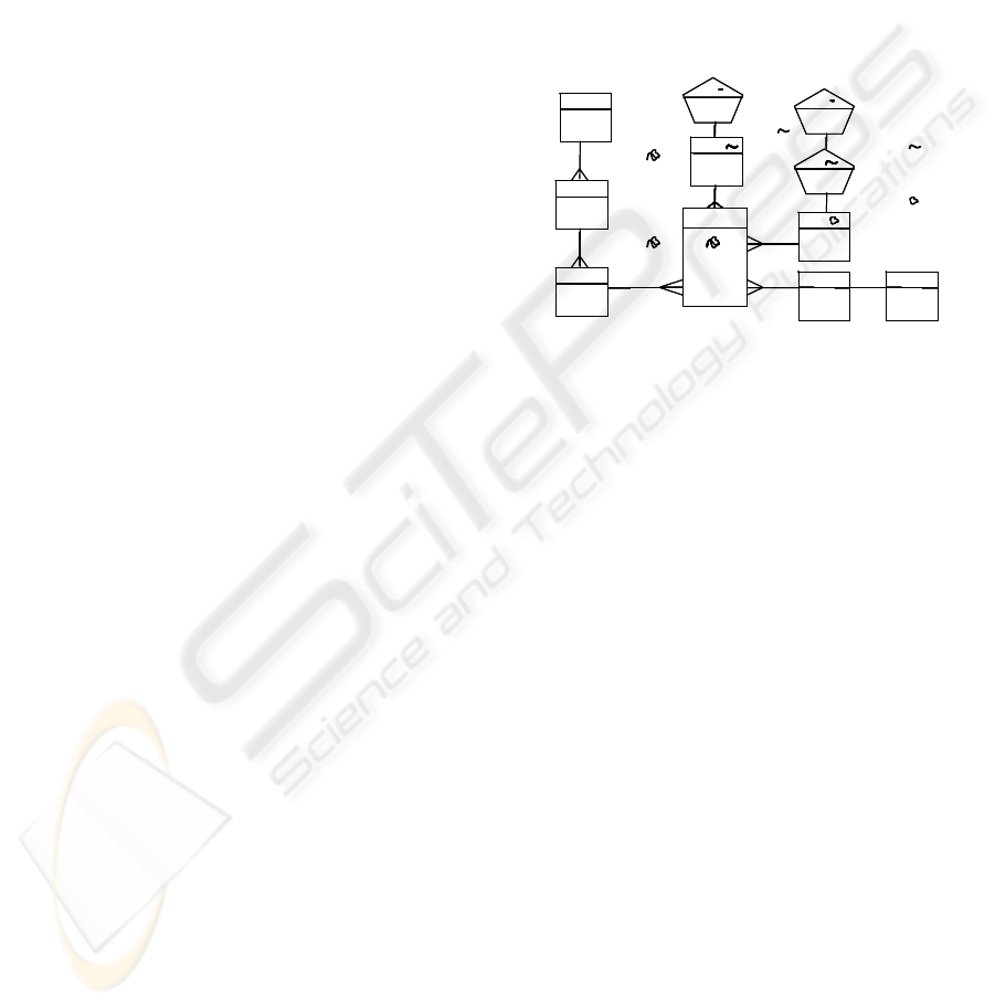
We show this example as Figure 4. We have
four dimensions: River Space, Plot Space, Location
and Time; and a fact table: Cross. In this scheme,
the topology functions are applied with two spatial
data, gathering the intersection or cross of two
different geometries, one for rivers and another for
surfaces of plots. The River Space Dimension has
two granularities, the less granularity (leaf level) is
represented with a lineal geometry show in metre
and the greatest granularity (second level) is show in
Hm unit associated to a point geometric. Plot Space
Dimension has three granularities, the less
granularity chosen is metre associated to a
polynomial representation, the second level has
hectometre unit associated to a geometric linear and
third level is represented as kilometre unit associated
to a geometric point. The Location dimension has
three levels: City, State and Country. The Time
dimension show by two granularities, month and
year, and has pre-established points in time. The
changes in the DW are made every month, and the
variations experienced by the different elements
present in the scheme, are only reflected at that time.
The Cross fact table has a measure that is the
intersection or crossing of the two spatial data, the
river spatial data and plot spatial data. The key of
this table is formed by the plot and river identities,
and also with the keys of the leaf levels of the
Location dimension and Time dimension.
In the Location dimension when Roll-up is
performed to reach a coarser granularity, the
aggregation function applied to the "intersection
(river, plot)" measure is the Union the same for all
levels. When Roll-up is done on the Time
dimension, in order to reach the coarser granularity
year, the M_last function, (Table 2,1) is applied to
“intersection (river, plot)” measure, and among all
the values of the spatial data of the granularity
months, we obtain at the end of every year. In the
River dimension to reach a coarse granularity from
the leaf level the Roll-up is applied and the Ml_contr
function is used on the river spatial attribute, which
reduces a line (m) to a point (Hm). In the Plot
dimension, the Roll-up applies the Mr_thinning or
Ml_contr function to the plot spatial attribute, which
reduces a region (m) to a line (Hm) or reduces a line
(Hm) to a point (km), respectively.
Each spatial element can change its granularity
independently of one another, and the intersection or
crossing between river spatial measure and plot
spatial measure can be performed through polygons
and lines, lines and points or across lines and lines, (
see Figure 4).
h
IDP m
IDR m
City_x
Month_x
City
State_x
Month
Month_x
Mr_thinning (IDP )
Ml_contr (IDP )
Hm
Km
Hm
IDR
Ml_contr (IDR )
h
Km
Hm
h
Km
Hm
h
Km
Hm
Location Dimension
Dynamic Hierarcy
Km
Hm
Cross
State
Country
City_x
Country_x
Union (IDP,IDR )
Plot Space Dimension
Static Hierarchy
Time
Dimension
Km
River m
Hm
IDP
M_Last (IDP, IDP )
Plot m
Year
Year_x
River Space Dimension
Static Hierarchy
Union ( IDP,IDR )
h
IDP m
IDR m
City_x
Month_x
City
State_x
Month
Month_x
Mr_thinning (IDP )
Ml_contr (IDP )
Hm
Km
Hm
IDR
Ml_contr (IDR )
h
Km
Hm
h
Km
Hm
h
Km
Hm
Location Dimension
Dynamic Hierarcy
Km
Hm
Cross
State
Country
City_x
Country_x
Union (IDP,IDR )
Plot Space Dimension
Static Hierarchy
Time
Dimension
Km
River m
Hm
IDP
M_Last (IDP, IDP )
Plot m
Year
Year_x
River Space Dimension
Static Hierarchy
Union ( IDP,IDR )
Figure 4: Example with more than one spatial dimension
present in the fact tables.
Example 3. We want study the evolution of the
plots whose variation is conditioned by the city to
which it belongs and by its owner, through time. We
want to store the plots as spatial data and its area
as numerical data. Also the timestamps included in
the DW will be motivated by the changes in
ownership and location of the plot, or in other
words, by events.
This example is modelled in Figure 5. In the fact
table we have two spatial measure focuses of study.
The Plot measure that gathers the evolution of the
plot through time and another Area measure, that
gathers the area of the plot in each evolution.
Although both of them are spatial data, the
characteristics and the treatment of them are differ;
Plot measure (represented by an identifier, a
geometry and a system of reference) and the Area
measure expressed in numerical form.
We believe that it is not necessary to have a spatial
dimension in order for a spatial measure to exist in
the fact table, nevertheless we propose that it be
included in the schema, when it is needed to treat
different granularities from a space object. Thus, we
introduce the Plot Space dimension associated to
Plot measure. Notice the intuitiveness of schema
when using the labels between the levels of
hierarchies to express the functions, applied to the
A MULTIDIMENSIONAL APPROACH TO THE REPRESENTATION OF THE SPATIO-TEMPORAL
MULTI-GRANULARITY
179
measures, when changing the granularities, i.e. when
the Roll-up is made, (Figure 5).
Evolution
IDP m
Area m
SSN
City_x
Time_x
State
Country
City
City_x
State_x
Country_x
Owner
SSN
Time
Time_x
Event_x
Union ( IDP )
Sum ( Area)
Union ( IDP )
Sum ( Area)
Mr_thinning (IDP )
Expre1(Area)
Ml_contr (IDP )
Expre2 (Area)
Plot Space Dimension
Static Hierarchy
Time
Dimension
Location Dimension
Dynamic Hierarcy
Owner Dimension
Hm
Km
Plot m
IDP
Evolution
IDP m
Area m
SSN
City_x
Time_x
IDP m
Area m
SSN
City_x
Time_x
IDP m
Area m
SSN
City_x
Time_x
IDP m
Area m
SSN
City_x
Time_x
State
Country
City
City_x
State_x
Country_x
OwnerOwner
SSN
Time
Time_x
Event_x
Time
Time_x
Event_x
Time
Time_x
Event_x
Union ( IDP )
Sum ( Area)
Union ( IDP )
Sum ( Area)
Mr_thinning (IDP )
Expre1(Area)
Ml_contr (IDP )
Expre2 (Area)
Plot Space Dimension
Static Hierarchy
Time
Dimension
Location Dimension
Dynamic Hierarcy
Owner Dimension
Hm
KmKmKm
Plot m
IDP
Figure 5: Example with a spatial data like a measure in
the fact table and one related measure.
6 CONCLUSIONS
In this paper we have described a novel approach to
extend multidimensional logical model using an
extension of the Snowflake scheme. Our objective is
the treatment of spatio-temporal granularity in the
multidimensional model. We have studied the
behaviour of spatial data when is included in a
dimension or in fact tables. Moreover, we have
shown the changes of spatio-temporal granularity in
spatial data, within a scheme which is clear and
intuitive. The Temporal dimension is presented with
a point of time pre-established and like time points
produced by events. We propose a new class of
hierarchy, called Static hierarchy, within the spatial
dimensions to gather the different granularities in a
chosen spatial reference system. The treatment of
the Static hierarchy is different from the treatment of
the hierarchies used until now by traditional
multidimensional models. The navigation through
the different levels of this Static hierarchy does not
imply changes in the measures of the fact tables, nor
in the spatial attributes inherited from a spatial
dimension, present in the key of the fact table.
Nonetheless the navigation through Static hierarchy
implies changes in the spatial representation of
spatial element that appear in the fact table, allowing
its study from different persperctives. We also
propose to place a label between the consecutive
levels of the hierarchies, with information of name
of function and with the measure which uses the
function when Roll-up is made on the hierarchies.
This clarifies and increases the semantic
representation of the scheme. Our future work focus
on including spatial objects in the multidimensional
model from a conceptual perspective, taking
advantage of the expressiveness that this offers to
derive a conceptual sheme independent from the
platform, the study of spatial data in movement and
the study of new static hierarchies searching for
more applications.
REFERENCES
Bettini, C., Jajodia, S. & Wang, S. “Time Granularities in
Databases, Data Mining and Temporal Reasoning”.
Springer-Verlag, 2000.
Camossi, E. Bertolotto, M. Bertino, E. Guerrini, G. A
Multigranular Spactiotemporal Data Model, GIS ‘03’
Eisenberg, A., Melton, J., Kulkarni, K., Michels, J.E.,
Zemke, F. “SQL: 2003 Has Been Published”.
SIGMOD Record, vol. 33, no. 1, March 2004.
Ferri F. Porurabbas, E. Rafanelli, M. and Ricci, F..
Extending geographic databases for a query language
to support queries involving statistical data. In Proc.
Of the 8th ACM Symposium on Advances in
Geographic Information Systems, 2000
Forlizzi, L., Güting, R.H., Nardelli, E., Schneider, M. “A
data model and data structures formoving objects
database”. Proceedings of the 2000 ACM SIGMOD
International Conference on Management of data, pp:
319-330, 2000.
Han, J. Koperski, K. and Stefanovic, N. GeoMiner: A
system prototype for spatial data mining. In Proc. Of
the ACM SIGMOD Int. Conf. On Managemente of
Data, 1997
Kouba, Z. Matou¡sek, K. and Mik¡sovský, P. Novel
knowledge discovery tools in industrial applications.
In Proc. of the Workshop on Intelligent Methods for
Quality Improvement in Industrial Practice, pages
72-83, 2002.
Malinowski, E. and Zimányi, E. Representing Spatiality in
a Conceptual Multidimensional Model. GIS’04,
November 2004, Washington, DC, USA.
Miquel, M. Brisebois, A. Bédard, Y. and Edwards, G..
Implementation and evaluation of hypercube-based
method for spatio-temporal exploration and anlysis.
SCG661 2004
Pourabbas. Cooperation with geographic database. In
Rafanelli[25], pages 393-432.
Rives, S. Bédar, Y. and Marchand, P. Toward better
support for spatial decision making: Defining the
characteristics of spatial on- line analytical
processing (SOLAP). Geomatica, 55 (4), 2001
Stefanovic, N. Han, J. and Koperski, K. Object-based
selective materializacion for efficiente implementacion
of spatial data cubes. IEEE Trans. On Knowledge and
Data Engineering, 12(6):938-958, 2000.
ICEIS 2006 - DATABASES AND INFORMATION SYSTEMS INTEGRATION
180
