
Virtual Remote Measurement of Controlled Sources
Florin Sandu, Gheorghe Scutaru,, Ioan Emilian Cucerzan, Daniel Iolu
”Transilvania” University – Bd. Eroilor nr. 29A – Brasov – ROMANIA
Abstract. A two level client-server development was performed by web layer
(to send remote measurement stimuli + simulation parameters) and workbench
layer – implemented under National Instruments “LabView” control. The test
bench equipment allows both programming of signals generation / acquisition
and PSpice simulation triggering. MS “FrontPage”- and Macromedia “Flash”-
based string concatenation and Intranet local links in the “Network
Neighbourhood” allow direct publishing of the web page that groups simulation
results with those of remote experiments.
1 Introduction
The present paper is a result of the „Leonardo da Vinci” Pilot Program
RO/01/B/F/PP141024 “Virtual Electro-Lab”, having as a main goal the Internet
publication not only of information but also of experimental resources [1]. High-tech
laboratory instruments can be accessed from any location (e.g. even from home) and
even on the move, for real test and measurement combined with analytical simulation-
emulation. After this remote-accessed measurement process and data tele-
transmission, mathematical post-processing of experimental data-bases, multi-criteria
comparison with theoretic calculus and results of complex simulation on behavioral
(and extendable) models complete the capabilities of the future e-University.
2 The Work-Bench
The experimental configuration is controlled by a Pentium PC (with MS Windows
2000), using National Instruments „LabView 6i” in a virtual instrumentation (VI)
system with Internet access. It runs in Continuous mode and is powered by an UPS.
3 Client-Server Architecture
Microsoft systems (Internet Explorer browsers, Front-Page for web-site development
etc.) were chosen for the implementation for Internet. At the Client level Web forms
were used to post stimuli and configurations towards the test bench.
Sandu F., Scutaru G., Emilian Cucerzan I. and Iolu D. (2004).
Virtual Remote Measurement of Controlled Sources.
In Proceedings of the First International Workshop on e-Learning and Virtual and Remote Laboratories, pages 44-51
DOI: 10.5220/0001151900440051
Copyright
c
SciTePress
At WorkBench Server level, the LabView program runs (in „Continuous” mode),
in an instrumentation-oriented implementation that processes the stimuli, controls the
automated measurement (whose results are incorporated in a .html file published by
the virtual instrument directly on the WebServer, by a simple local link (in „Network
Neighbourhood”) – avoiding in this way expensive solutions such as „Internet
Toolkit” for LabView (with extra problems of specific methods – e.g. „Real-Time
Engine” – incorporation at Client level).
4 LabView programming at work-bench server level
We have implemented all four types of controlled sources: the Voltage Controlled
Voltage Source (VCVS), the Voltage Controlled Current Source (VCCS), the Current
Controlled Voltage Source (CCVS) and the Current Controlled Current Source
(CCCS). In the following it will be presented the structure of the VI that implements
only one of the above-mentioned source types, the VCCS and they will be detailed the
most important diagrams of this experiment's VI.
The VI consists of five frames, which are executed sequentially (from frame 0 to
frame 5). On the workbench server LabView is running in “continuous” mode
providing in this way an infinite loop.
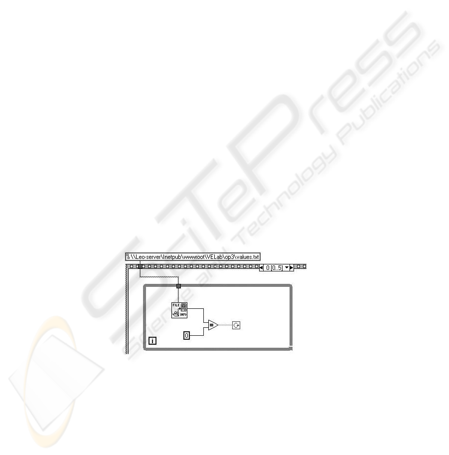
The first frame (fig. 1) contains a wait - loop in which we test if the stimuli file is
empty (this file is empty if no forms were posted). If the stimuli are posted, with a
mouse click on the “SUBMIT” button in the experiment’s control page, the step-out
from the loop continues with the frame 2. In this frame the last measurement input
and output files, that contain stimuli of measured values, are deleted.
The next frame (fig. 2) is extracting the variables from the stimuli file and
constructs the “.cir” file for PSpice simulation. In order to obtain the needed variables
for the construction of the “op3.cir” file, the stimuli file was preformatted on the
server using PHP. The stimuli file format is: “VarName:value\n …”.
Fig. 1. First frame of the VI, containing a wait – loop
43
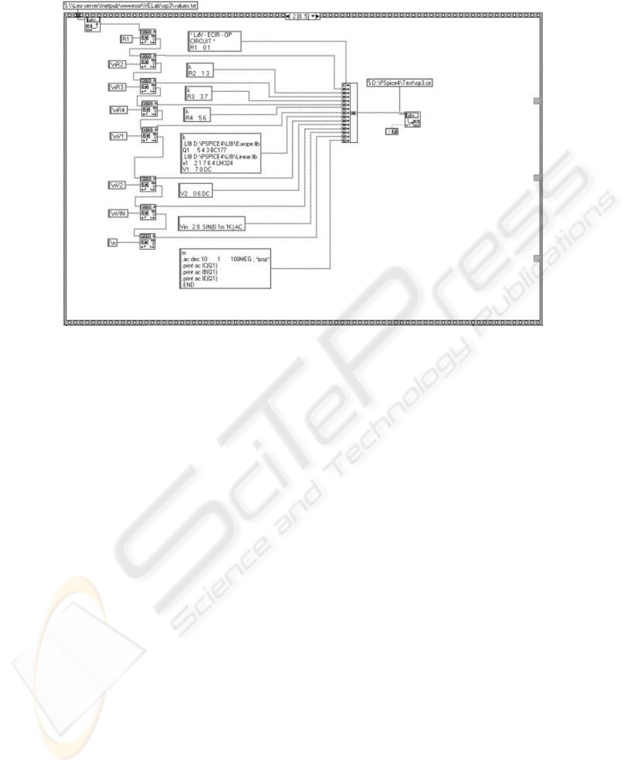
Fig. 2. Variables' extraction from the stimuli file and construct of the “.cir” file
The 3
th
frame contains a “System-exec” subVI, which launches the PSpice (on the
workbench server) having as parameter the name of the pre-constructed “op3.cir” file.
Next frame (fig. 3): creates the file that will be used on the client's machine to
generate the nodes' voltages (“op3_val.txt”); constructs three arrays used to plot
IC(frequency), IB(frequency), IE(frequency) graphs; deletes the stimuli file; writes
the output file(created on the work-bench machine as the result of PSpice simulation)
on the server. The blocks from the top of the VI frame (shown in figure 3) are
responsible for the construct of “op3_val.txt”. This part of the VI reads all characters
from “out.txt” file and writes them to “op3_val.txt” by replacing some character
strings (e.g.: “( 2)” -> “&VP2”). The 3 similar blocks from the centre of the figure
create the arrays used for graphics plot. The arrays values are extracted from
“op3.out” using string identification blocks (to identify the beginning line) and by
knowing the exact position of the frequency and current values (which form an array
element) on each line in the “op3.out” file. The number of lines is 81 (this constant is
given as the result of simulation request).
Last VI frame (fig. 4) displays the 3 graphics and saves their controls (containing
the graphics images) as JPG files. The controls' save to JPG was made by adding an
invoke node (contains “GetImage” function) to the graphic control and by using the
“JPG save” subVI.
The “image file save” part was separated from the graphics arrays construct part to
avoid the saving of older graphics images. The graphic is displayed on the graphic
control only when the graphic array construction was finally accomplished. If the
“image file save” part would be included in the frame 4, it would have been possible
that the image from the graphic control should be saved before the control re-
actualisation.
44
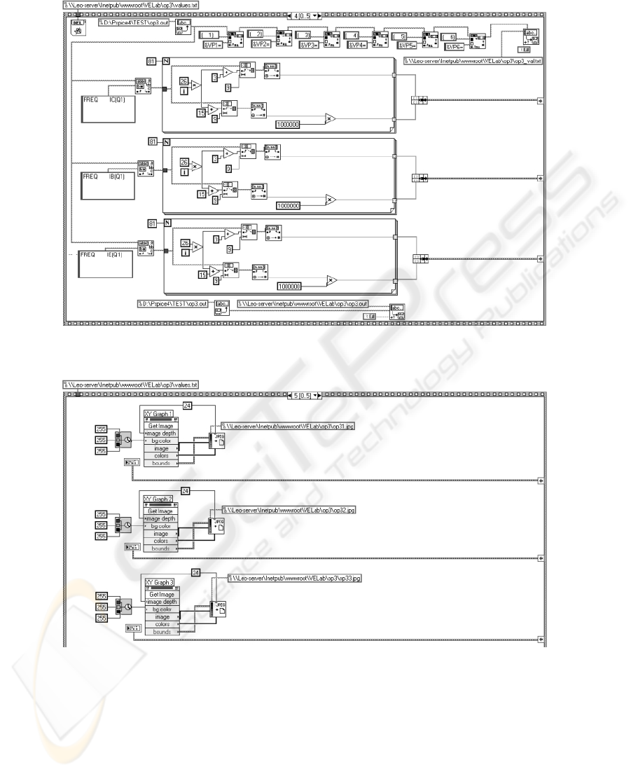
Fig. 3. Frame 4 of the VI, containing the construction of the“op3_val.txt” file, the graphics
arrays construction and the copy of op3.out from the work-bench to server
Fig. 4. Graphics plot and image-to-file save frame
When the VI execution reaches frame 5, the VI will continue to run from frame 1
providing this way an infinite loop.
45
5 PSpice Simulated Hyper-Schematic
In order to create an easy-to-use interface for the triggering of remote PSpice
simulation and spectacular retrieval of the results directly to/from a “hyper-
schematic” (on which the user can directly change parameters and observe bias points
in a very intuitive way) we have used FLASH 5 from MACROMEDIA. Our choice is
justified by the multiple advantages it offers:
- Vector graphics (zoom without loosing quality)
- Easy editing (in a graphical editing environment)
- Scripting language (“Action Script”)
- Capabilities for communication with other files (the own variables can be
transmitted in both ways to/from a file)
Our aim was to create a “user friendly” interface (with edit boxes near the symbol
of “hyper-schematic” devices whose associated value should be variable) and to
return the results in the same schematic. Using FLASH 5 proved to be a good choice
for this interface.
(a)
(a) (b)
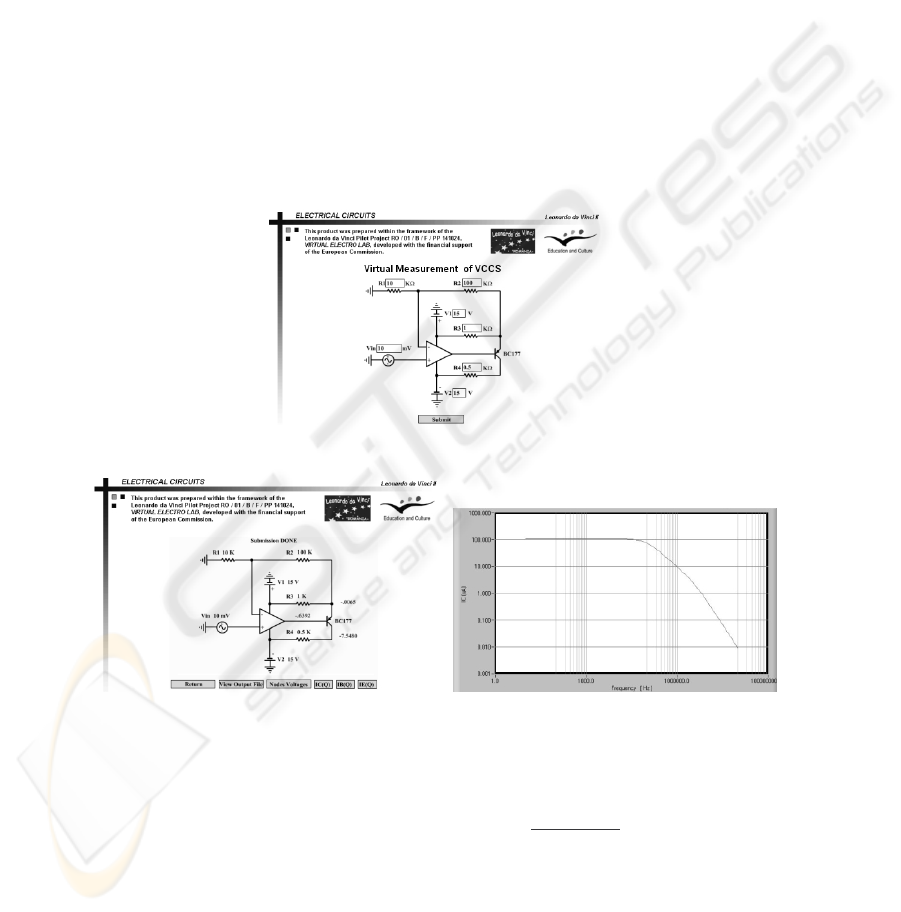
Fig. 5. – VCCS "hyper-schematic" on a course "page"
(a) – text boxes for numerical submission (with default values)
(b) – the node voltages (the student can notice the correct Bias-Point of the BJT)
(c) – plot of the
()
4434421
321
factordivider current of inverse
3
R
3
R
2
R
1
R
1
R
I AC
1
G
in
V I AC
c
⎟
⎠
⎞
⎜
⎝
⎛
++
⋅⋅=
46

For the accomplishment of the associated .SWF” movie, graphics and scripting
were merged together. First the schematic was designed and then edit boxes were
added (Fig.5a).
Our movie-interface is structured in a single scene, 2 layers and 4 frames.
The first layer serves for actions (programming), and the second one for graphics. In
the first frame the initialization is made; the second frame contains the input part of
the application; in the 3rd frame are checked and enabled the data that were input in
frame 2; the 4th frame contains the outputs (in this part are displayed the results of the
simulation – see fig.5b and 5c).
The Functions Used for the Implementation are:
LoadVariablesNum ("http://vlab.unitbv.ro/VELab/op3/op3.php", 0, "POST"); that
sends variables form level 0 of the movie, using POST method, to op3.php file
LoadVariablesNum ("http://vlab.unitbv.ro/VELab/op3/op3_val.txt", 0); that reads
data from an external file (op3_val.txt), assembled by the VI (fig.6) and sets the
values for variables in movie. In the file 'op3_val.txt' the variables must be defined
like variable name=value and separated with '&'. The variable name from the external
file must be the same with the variable name inside the movie.
GetURL("http://vlab.unitbv.ro/VELab/op3/op3.out", "_blank"); that loads a document
from a specific URL into a window. This function is used in order to view 'op3.out',
'op31.jpg', 'op32.jpg' and 'op33.jpg' files.
gotoAndPlay(4); that sends the play head to the frame 4 and plays from that frame
gotoAndStop(4) ; that sends the play head to the frame 4 and stops it
stop(); that stops the movie currently playing
In order to create the 'values.txt' file we have used the server side scripting
language PHP (provided for free). The FLASH function loadVariablesNum
("http://vlab.unitbv.ro/VELab/op3/op3.php", 0, "POST") calls the op3.php file and
passes to it, through POST method, all the variables from the movie level 0.
"op3.php" has the role to over-take these variables and to write them, according to a
preset format, in the values.txt file.
Here it is the commented op3.php listing:
<?php
//gets all variables from swf file
$vin = $HTTP_POST_VARS['vin'];
$r1 = $HTTP_POST_VARS['r1'];
$r2 = $HTTP_POST_VARS['r2'];
$r3 = $HTTP_POST_VARS['r3'];
$r4 = $HTTP_POST_VARS['r4'];
$v1 = $HTTP_POST_VARS['v1'];
$v2 = $HTTP_POST_VARS['v2'];
//create and open the output file
$filename="./values.txt";
if (!file_exists($filename)) {
touch($filename);
// Create blank file
chmod($filename,0666);
}
$f=fopen($filename,"w");
//writes input values in the file
//"values.txt"
fputs($f,"R1:".$r1."\n");
fputs($f,"R2:".$r2."\n");
fputs($f,"R3:".$r3."\n");
fputs($f,"R4:".$r4."\n");
fputs($f,"V1:".$v1."\n");
fputs($f,"V2:".$v2."\n");
fputs($f,"VIN:".$vin."\n");
fclose($f);
?>
47
6 Practical student works on the four hyper-circuits
The simplest configuration (without the need of any auxiliary components or of any
conversion) is the VCVS (fig. 6):
(a) (b)
(c)
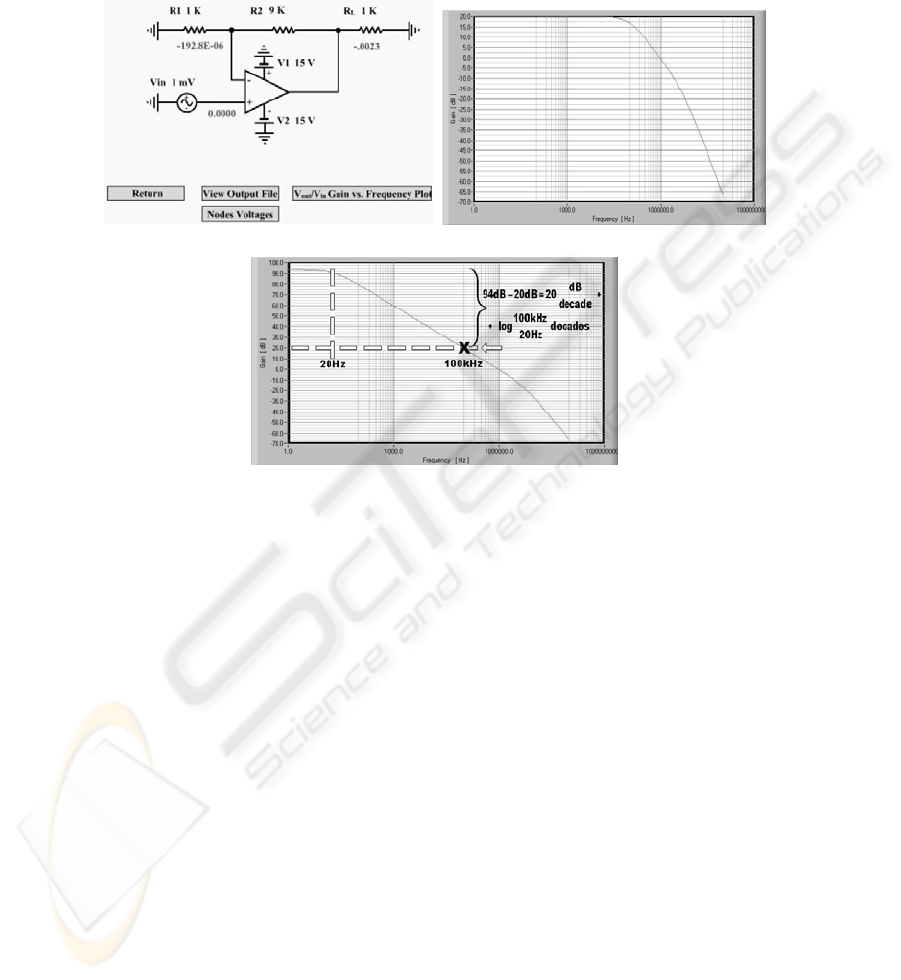
Fig. 6. VCVS – Schematic with a particular set of values
(a) The display of node voltages; (b) The gain plot
(c) Cuasi-open loop gain as reference for auxiliary graphical construction
The student can check (fig. 6b) the in-band value (1 + R
2
/ R
1
) = 20 dB, the
particular value of approx. 100 kHz for the upper -3dB frequency, on the –
20dB/decade slope, the second pole (data-sheet value, practically independent of the
particular feed-back) of approx. 5 MHz and the change of slope to –40dB/decade.
The cuasi-open loop gain plot (fig. 6c) - obtained with largest value of R
2
/R
1
ratio and
extremely small V
in
that keeps the signal between the limits of the power supplies -
can serve as reference for finite gains ( 1 + R
2
/ R
1
) equal to the inverse of the
negative feed-back factor (the open-loop gain is actually of approx. 106 dB, with the
first pole at approx. 5Hz). The student can trace auxiliary lines that enable the check
of the increase of -3dB upper frequency exactly as many times the gain decrease.
The CCVS (fig.7) is actually a trans-impedance negative feed-back amplifier (gain
equal to – R
2
) with the input current converted by R
1
from an alternative voltage
source; it results the proper input AC V
in
/ R
1
(and the indirect voltage gain –R
2
/R
1
).
The CCCS (fig. 8) is using the same input current conversion (V
in
/ R
1
) and the
adapted basic VCCS configuration (see also the CCVS similarity to VCVS).
The core schematic is built around LM324 that drives the base of BC177 BJT.
48
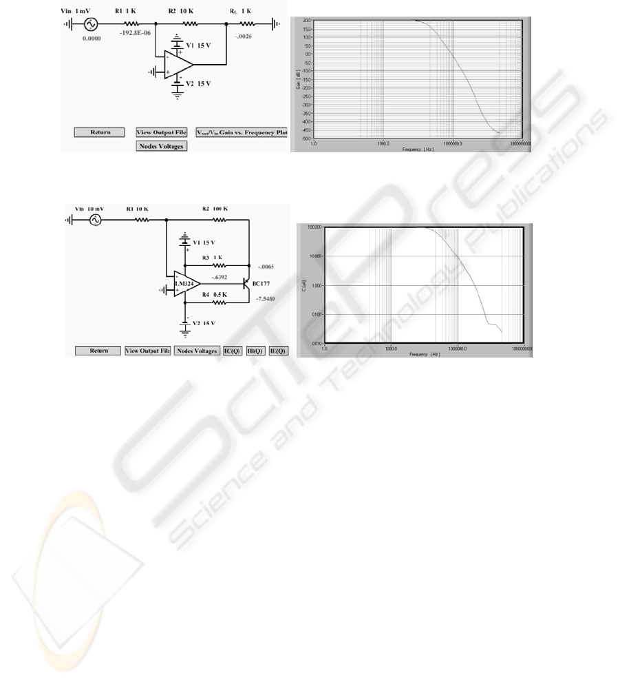
It also accomplishes full overtake of the input current by R
2
and clamping R
2
left
terminal to ground so it will build an (adjustable – by R
2
) alternative current divider
with R
3
(the proper AC gain is then I
R4
/ I
R1
= 1 + R
2
/R
3
). R
3
plays also a DC role, to
bias BC177, together with R
4
- this also plays a double role, being, for AC, a current-
to voltage transducer, for (practical) measurement of the output.
(a) (b)
Fig. 7. CCVS – Schematic with a particular set of values
(a) The display of node voltages; (b) The (–) R
2
/R
1
gain plot
(a) (b)
Fi
g. 8. CCCS – Schematic with a particular set of values
(b) The display of node voltages; (b) The gain plot
7 Conclusions
Authors' work aimed to fill a gap between the written course and practical (remote)
measurement: simulation-emulation was integrated in a more friendly eBook, running
on the same work-bench server that will be accessed by the student for the
experiments. The results can be extended, due to larger models' libraries available
(also extendable by behavioural modelling) e.g. to electro-mechanical automation &
robotics, with an implementation that should also include virtual reality.
References
1. F. Sandu, W. Szabo, P.N. Borza, "Automated Measurement Laboratory Accessed by
Internet", in Proc. of the XVI IMEKO World Congress 2000, Vienna, Austria.
2. I. Szekely, J. Goes, C. Gerigan, G. Pana, C. Stanca, "Measurement of Electronic Devices
and Circuits", Ed. Lux Libris, Brasov, 2003, ISBN 973-9428-96-9.
49
