
HYBRID CONTROL DESIGN FOR A ROBOT MANIPULATOR
IN A SHIELD TUNNELING MACHINE
Jelmer Braaksma, Ben Klaassens, Robert Babu
ˇ
ska
Delft Center for Systems and Control, Delft University of Technology
Mekelweg 2, 2628 CD Delft, the Netherlands
Cees de Keizer
IHC Systems B.V., P.O. Box 41, 3360 AA Sliedrecht, the Netherlands
Keywords:
Robotic manipulator, shield tunneling, hybrid control, collision, environment model, feedback linearization.
Abstract:
In a novel shield tunneling method, the tunnel lining is produced by an extrusion process with continuous
shield advance. A robotic manipulator is used to build the tunnel supporting formwork, consisting of rings
of steel segments. As the shield of the tunnel-boring machine advances, concrete is continuously injected in
the space between the formwork and the surrounding soil. This technology requires a fully automated ma-
nipulator, since potential human errors may jeopardize the continuity of the tunneling process. Moreover, the
environment is hazardous for human operators. The manipulator has a linked structure with seven degrees of
freedom and it is equipped with a head that can clamp the formwork segment. To design and test the controller,
a dynamic model of the manipulator and its environment was first developed. Then, a feedback-linearizing hy-
brid position-force controller was designed. The design was validated through simulation in Matlab/Simulink.
Virtual reality visualization was used to demonstrate the compliance properties of the controlled system.
1 INTRODUCTION
With conventional shield tunnel boring machines
(TBM), the tunnel lining is built of pre-fabricated
concrete segments (Tanaka, 1995; K. Kosuge et al.,
1996). These segments must be transported from the
factory to the construction site, which requires con-
siderable logistics effort. Delays in delivery and dam-
age of the segments during their transport are not un-
common.
To improve the process, IHC Tunneling Systems
are developing a novel shield tunneling method in
which the tunnel lining is produced by extruding con-
crete in the space between the drilled hole and the
supporting steel formwork. This formwork is built of
rings, each consisting of eight segments.
The main functions of the formwork are: i) sup-
port the extruded concrete tunnel lining until it is
hardened and becomes self-supporting, ii) provide the
thrust force to the TBM shield which actually exca-
vates the tunnel. The thrust is supplied by 16 indi-
vidually controlled hydraulic thrust cylinders, evenly
spread around the shield’s circumference.
A robotic manipulator (erector) is used to place the
segments at the desired position. The erector is a
linked robot mounted such that it can rotate around
the TBM spine, see Fig. 1. It is equipped with a head
that clamps the segment and picks it up from the con-
veyer. At the back end of the TBM, the concrete is al-
ready hardened and the formwork can be dismantled
by a similar manipulator (derector). The segments
are cleaned and inspected for possible damage before
they can be transported to the front end of the TBM
and re-used.
As in the proposed method the tunnel-boring pro-
cess is continuous (maximum speed of 2 m/h), the
segments have to be placed within a limited time
interval, and simultaneously with the TBM forward
movement. To comply with the stringent timing re-
quirements and to ensure the continuity of the boring
process, the erector must be controlled automatically
(as opposed to the current practice of using operator-
controlled manipulators). By automating the process,
the probability of a human error is limited and also
the hazard for the operator is considerably reduced.
The controller of the erector must guarantee stable
and safe operation in three different modes (Fig. 2):
1. The segment is in free space and the main task is to
bring it close to the desired position.
2. The segment is in contact with the hydraulic thrust
cylinders which push it toward the already placed
formwork ring.
185
Braaksma J., Klaassens B., Babuška R. and Keizer C. (2004).
HYBRID CONTROL DESIGN FOR A ROBOT MANIPULATOR IN A SHIELD TUNNELING MACHINE.
In Proceedings of the First International Conference on Informatics in Control, Automation and Robotics, pages 185-192
DOI: 10.5220/0001128901850192
Copyright
c
SciTePress
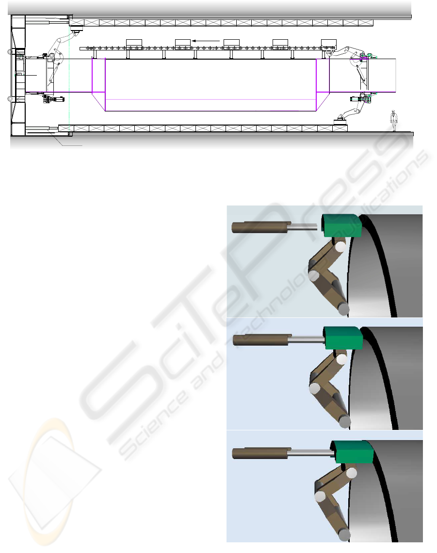
erector
conveyer
derector
formwork
hydraulic thrust cylinders
spine
shield
concrete
Figure 1: Cross-section of the shield tunneling machine. Two working configurations of the derector are shown.
3. The segment is in contact with the hydraulic thrust
cylinders and the formwork ring. The force deliv-
ered by the thrust cylinders will align the segment
in the desired position.
While the first mode is characterized by traditional
trajectory-following control, the latter two modes re-
quire compliant control, capable of limiting the con-
tact forces and correcting a possible mis-alignment
due to a different orientation of the segment and the
already placed ring. Note that no absolute measure-
ment of the segment position is available, it can only
be indirectly derived from the measurements of the
individual angles of the manipulator links.
To analyze the process and to design the control
system, a detailed dynamic model of the erector has
been developed. This model includes collision mod-
els for operation modes 2 and 3. A hybrid control
scheme is then applied to control certain DOFs by
a position control law and the remaining ones by a
force control law. Input-output feedback linearization
is applied in the joint space coordinates. Simulation
results are reported.
2 MODELING
The mathematical model consists of three parts: the
manipulator, the environment and the hydraulic thrust
cylinders. This section describes these elements one
by one.
2.1 Manipulator model
The erector was designed as a linked structure with
three arms and a fine-positioning head, see Fig. 3. The
first arm is attached to the base ring (body0) that can
rotate around the spine. This ring is actuated by an
electric motor. The arms are actuated by hydraulic
Hydraulic push actuators
Manipulator
Segment to be placed
Ring, already built
Figure 2: The erector manipulates segments in three differ-
ent modes: in free space (top), in contact with the hydraulic
thrust cylinders (middle), in contact with the trust cylinders
and the segment ring (bottom).
ICINCO 2004 - ROBOTICS AND AUTOMATION
186

actuators (not modeled here). At the top of the third
arm (body3), the head is attached, which has three de-
grees of freedom (DOF). The entire manipulator has
seven DOF (q
0
to q
6
) in total.
q
2
q
0
q
1
q
3
(pitch)
q
6
(yaw)
q
5
(roll)
q
4
y
x
z
Spine
body2
body1
body0
body3
head
Figure 3: The structure and the corresponding degrees of
freedom of the erector.
The bodies are assumed rigid bodies and the DOF
in body0 is not taken into account. This is justified,
as the rotation around the spine is fixed during the
positioning of the head. Angle q
0
is still an input to
the model, fixed to a value between 0 and 2 π rad. The
control inputs of the robot are assumed to be perfect
torque/force generators in the joints.
The dynamic equation for the manipulator is:
D(q)
¨
q + C(q,
˙
q)
˙
q + F
v
˙
q + φ(q) = τ − J
b4
0
(q)
T
f
(1)
where f is the vector of contact forces between the
hydraulic thrust cylinders and the segment plus the
contact forces between the segment and the ring. The
matrix D(q) is the inertia matrix, C(q,
˙
q) is the Cori-
olis and centrifugal matrix, F
v
is the friction matrix
and φ(q) is the gravity vector. J
b4
0
is the Jacobian
from frame b4 to frame 0, and q is the vector of the
joint angles. The manipulator is actuated with the
torque/force vector τ .
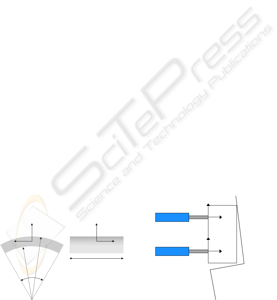
2.2 Environment model
The environment consists of the segment ring (Fig. 4).
An accurate environment model, very important to
the contact tasks in robotics, is usually difficult to
obtain in an analytic form. In the literature, usu-
ally a simplified linear model is used (Vukobratovi
´
c,
Figure 4: Two consecutive rings of the formwork. Each ring
consists of eight segments.
1994). The environment is modeled as a mass-spring-
damper-system. The surface of the segment’s side is
considered flat and only the normal force acting on the
side of the segment is taken into account. Tangential
friction forces are neglected. The collision detection
is implemented with the following smooth switching
function
g(x) =
1
π
atan(α(x − x
e
)) +
1
2
(2)
where α is the steepness of the function, x is the po-
sition of the segment and x
e
is the position of the en-
vironment. The environment force is described by the
following equation:
f
e
= g(x)(K
e
(x − x
e
) + D
e
( ˙x − ˙x
e
)) (3)
For stationary environments, equation (3) can be sim-
plified by taking ˙x
e
= 0. K
e
is the stiffness and D
e
is the damping.
hydraulic
push actuators
COG
f
e
f
l
segment
formwork ring
{ }C
a1
r
{ }C
a2
f
l
Figure 5: Decomposition of contact force f
e
.
In the Cartesian space, the dynamic behavior de-
pends on the direction vector of the force and the lo-
cation of the collision. Fig. 5 shows an unaligned col-
lision of the segment with the formwork ring. In this
HYBRID CONTROL DESIGN FOR A ROBOT MANIPULATOR IN A SHIELD TUNNELING MACHINE
187
figure, a transformation is applied, which decomposes
a force f
e
into a force f
l
and torque τ acting on the
center of gravity (COG). The following formulas can
be applied.
f
l
= f
e
(4)
τ = r × f
e
(5)
where r points to the place where the force acts. The
above derivation is valid for a body moving in free
space. The transformation of the force and torque to
the joint torque is achieved using the principle of vir-
tual work, see (Spong and Vidyasagar, 1989). The
following formula for the joint torques can be derived
τ
e
= J
0
(q)
T
·
R
b4
0
0
0 R
b4
0
¸
f with f =
·
f
l
τ
¸
(6)
where R
b4
0
transforms the force expressed in the seg-
ment body frame to the base frame, J
0
(q) is the Ja-
cobian which transforms the joint speeds to the lin-
ear/rotational speeds in the base frame and τ
e
is a
vector with joint torques/forces.
2.3 Hydraulic thrust cylinders
The model consists of a collision model and a hy-
draulic model. The collision model must detect the
collision between the hydraulic thrust cylinders and
the formwork ring, which means that the model must
detect whether the tips are contacting the segment
body (body4). If there is a collision, the magnitude of
the force can be calculated with the scheme explained
in Section 2.2.
The shape of a segment is illustrated in Fig. 6. The
segment (body4) is a part of a hollow cylinder. For
a controlled collision, the y coordinate of tip of the
hydraulic thrust cylinders must be between the inner
radius r
1
and the outer radius r
2
, and within the range
ϕ, see Fig. 6. The kinematic transformation of two
hydraulic thrust cylinders tips to the C
b4
frame is used
to detect collision.
x
b4
{C
b4
}
z
b4
r
1
r
2
j
x
b4
z
b4
y
side view
body4
Figure 6: The dimensions of the segment (body4).
When the actuators come into contact with the seg-
ment, this will result in a force and torque as ex-
plained in Fig. 5. Only the normal force acting on the
segment is simulated. The error between the segment
and the thrust cylinders is at most 3 degrees, satisfying
the assumption to neglect the tangential force. The
force and torque in the C
b4
frame, are calculated with
the following equations. Let H
b4
a1
and H
b4
a2
be the ho-
mogeneous transformations from the thrust cylinder
frames (C
a1
, C
a2
) to C
b4
. The two force and torque
vectors can be calculated as follows
f
a1
= |f
a1
|[0 1 0]
T
r
a1
= (H
a1
b4
[0 0 0 1]
T
)
123
τ
a1
= r
a1
× f
a1
(7)
f
a2
= |f
a2
|[0 1 0]
T
r
a2
= (H
a2
b4
[0 0 0 1]
T
)
123
τ
a2
= r
a2
× f
a2
. (8)
where the subscript 123 refers to the first three ele-
ments. These forces and torques in the body frame
can be transformed to the joint torques by means of
the principle of virtual work (6).
3 HYBRID CONTROLLER
The manipulator in free space is position controlled,
but when it is in contact with the environment, the lat-
eral motion and rotation become constrained. When
the segment is pushed by the hydraulic thrust cylin-
ders, stable contact between the thrust cylinders and
the segment is maintained by controlling the contact
force (Fig. 7). When the segment comes into contact
with the segment ring, it aligns to the desired orienta-
tion and position. During the transition between the
modes it is required that the contact forces are lim-
ited. An impedance controller gives the manipulator
the desired compliant behavior (Hogan, 1985).
Hydraulic
push
actuators
y
c
y
c
z
c
z
c
Segment
Segment
ring
{C
a1
}
{C
a2
}
Figure 7: Top view of the segment.
ICINCO 2004 - ROBOTICS AND AUTOMATION
188

A control scheme known as a hybrid position force
controller of (Raibert and Craig, 1981) allows to spec-
ify for each DOF the type of control. The frame in
which the segment is controlled is positioned such
that the direction, in which the position is controlled,
is perpendicular to the direction in which the force is
controlled. This frame is called the constraint frame.
In our case the constraint frame is aligned with the
two thrust cylinder frames (see Fig. 7). In this sit-
uation, the yaw, y, and the pitch, z, DOFs are con-
strained. We choose for the y degree of freedom a
force controller to assure contact. For the other po-
sition constrained degrees of freedom an impedance
controller is chosen which guarantees compliant be-
havior.
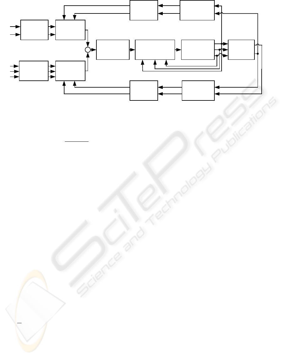
The controller consists of four blocks: feedback
linearization, transformation of sensor data (kinemat-
ics, Jacobian and coordinate transform), selection ma-
trix and the controllers (see Fig. 8).
The coordinate-transform block transforms the data
f, x, R, v and ω from the base frame to the constraint
frame and vice versa, where f is the measured force, x
is the position of the segment, R is the rotation matrix
which defines the orientation of the segment, v is the
linear speed of the segment and ω is the angular speed
of the segment. The inputs of the force controller are
f
d
and
˙
f
d
, which are the desired force and it’s deriva-
tive. The inputs of the position controller are x
d
,
˙
x
d
and
¨
x
d
, which are the desired position, velocity and
acceleration respectively. The vector a is the resolved
acceleration vector and τ is the torque/force vector
for the manipulator.
3.1 Feedback linearization
The following controller is used for feedback lin-
earization (Siciliano and Villani, 1999)
τ =
ˆ
D(q)u +
ˆ
C(q,
˙
q)
˙
q +
ˆ
F
v
˙
q +
ˆ
φ(q) + J
b4
0
(q)
T
f
(9)
where u is the new acceleration control input. Sub-
stituting (9) into (1) and assuming perfect modeling
results in the following system
¨
q = u (10)
The goal of the controller is to control the manipulator
in the constraint frame to its desired values.
The Jacobian transforms the joint velocities to the
linear and rotational speeds. The Jacobian is given by
·
v
b4
0
ω
b4
0
¸
= J
b4
0
(q)
˙
q (11)
Differentiating (11) gives
·
˙
v
b4
0
˙
ω
b4
0
¸
=
¨
x = J
b4
0
(q)
¨
q +
˙
J
b4
0
(q)
˙
q (12)
which represents the relationship between the joint
acceleration and the segment’s linear and rotational
speed. A new control input can now be chosen as
u = (J
b4
0
(q))
−1
³
a −
˙
J
b4
0
(q)
˙
q
´
. (13)
Substitute (13) into (10) and the result into (12), as-
suming perfect modeling and perfect force measure-
ment, leads to the following total plant model
¨
x = a = a
p
+ a
f
(14)
where a is the resolved acceleration in the base frame
and a
p
, a
f
are the outputs of the position controller
and force controller in the base frame. The vector a
p
can be partitioned into linear acceleration a
l
and an-
gular acceleration a
o
. Likewise, a
f
can be partitioned
into linear acceleration a
fl
and angular acceleration
a
ft
:
a
p
=
·
a
l
a
o
¸
a
f
=
·
a
fl
a
ft
¸
. (15)
3.2 Transformation of sensor data
The different positions and speeds are measured in the
joints of the manipulator. The force is measured us-
ing a force sensor, located in the manipulator head. To
control the manipulator in Cartesian space these mea-
surements must be transformed to a Cartesian frame.
This is done with the kinematic matrix and the Jaco-
bian matrix. The frame in which the manipulator is
controlled is the constraint frame.
3.3 Selection matrix
The DOF for position control and for force control
can be selected. This is done by multiplying the
force/torque vector by a diagonal selection matrix S
and the position/velocity vector by I − S, with I the
identity matrix. For a DOF that is position controlled
S
i
= 0 and for a force controlled DOF S
i
= 1. For a
manipulator moving in free space the selection matrix
is a zero matrix, meaning position control.
To make sure that the switch between the two sit-
uations is in a controlled manner, the switch function
of the selection matrix must be smooth. The time of
switching in unknown, so the switch should be trig-
gered by the contact force (Zhang et al., 2001).
Φ
i
(f
i
) =
½
f
i
− f
i
ref 1
, if f
i
≥ 0
f
i
ref 2
− f
i
, if f
i
< 0
(16)
The smooth switch function can now be defined as
S
i
=
½
0, if Φ
i
(f
i
) < 0
1 − sech(αΦ
i
(f
i
)), otherwise
(17)
HYBRID CONTROL DESIGN FOR A ROBOT MANIPULATOR IN A SHIELD TUNNELING MACHINE
189
Feedback
linearization &
Cartesian to joint
space transformation
Coordinate
transform
Manipulator
+
Environment
Coordinate
transform
Position
controller
Selection
matrix
Selection
matrix
Force
controller
Coordinate
transform
Kinematics
+
Jacobian
Selection
matrix
Selection
matrix
f
x
,
R
v
,
w
+
+
t
q
.
q
a
f
d
.
f
d
..
x
d
.
x
d
x
d
Figure 8: Block diagram of the hybrid position force controller.
with
sech(x) =
2
e
x
+ e
−x
(18)
The value α determines the steepness of the curve,
and f
i
ref 1
, f
i
ref 2
are the upper and lower threshold
values respectively. The steepness α should be chosen
such that the S
i
= 1, when the desired contact force
is reached. The force in the y DOF (in the constraint
frame) is chosen to switch from position control to
force/impedance control.
3.4 Position control
For the linear and decoupled system (14), the follow-
ing control can be used in order to give the system the
desired dynamics (Siciliano and Villani, 1999).
a
l
=
¨
x
d
+ D
l
(
˙
x
d
−
˙
x) + P
l
(x
d
− x) (19)
a
o
=
˙
ω
d
+ D
o
(ω
d
− ω) + P
o
R
c
b4
²
d
b4
(20)
This is a PD controller for the position controlled
DOF, where R
c
b4
transforms the quarternion error ²
d
b4
from the C
b4
frame to the constraint frame. The ma-
trices D
l
and D
o
are the diagonal damping matri-
ces, and P
l
and P
o
are the proportional gain matrices.
Substituting (19) and (20) into (14) assuming perfect
modeling gives the total plant model
¨x =
S
·
¨x
d
+ D
l
( ˙x
d
− ˙x) + P
l
(x
d
− x)
˙
ω
d
+ D
o
(ω
d
− ω) + P
o
R
e
2
²
de
e
¸
(21)
3.5 Force control
The force controller has an inner position/orientation
loop within the force loop. For the position loop, the
following PD-controller is chosen (Siciliano and Vil-
lani, 1999).
a
f
= −D
f
˙
x + P
fp
(x
c
− x) (22)
where x
c
− x is the difference between x
c
the
output of the force loop and the measured posi-
tion/orientation x and P
fp
is the proportional matrix
gain and D
f
is damping gain. For the force loop a
proportional-integral (PI) control is chosen
x
c
= P
−1
fp
µ
P
f
(f
d
− f ) + P
I
Z
t
0
(f
d
− f )dς
(23)
where P
f
is the proportional gain, P
I
is the inte-
gral gain, f
d
is the desired force and f is the measured
force. The P
−1
fp
in (23) has been introduced to make
the resulting force and moment control action in (22)
independent of the choice of the proportional gain on
the position and orientation.
3.6 Impedance control
For the impedance controlled DOF the following con-
trol law can be chosen (Siciliano and Villani, 1999)
a
f
=
·
¨
x
d
+ M
−1
li
(D
li
(
˙
x
d
−
˙
x) + P
li
(x
d
− x) − f
l
)
˙
ω
d
+ M
−1
oi
(D
oi
(ω
d
− ω) + P
oi
R
c
b4
²
d
b4
− f
t
)
¸
(24)
with M
li
and M
oi
positive definite matrix gains,
leading to
M
li
(
¨
x
d
−
¨
x) + D
li
(
˙
x
d
−
˙
x) + P
li
(x
d
− x) = f
l
(25)
M
oi
(
˙
ω
d
−
˙
ω) + D
oi
(ω
d
− ω) + P
oi
R
c
b4
²
d
b4
= f
t
(26)
Equations (25) and (26) allow specifying the manipu-
lator dynamics through the desired impedance, where
the translational impedance is specified by M
li
, D
li
and P
li
and the rotational impedance is specified by
M
oi
, D
oi
and P
oi
.
ICINCO 2004 - ROBOTICS AND AUTOMATION
190
3.7 Simulation results
The rotation around the spine is fixed during fine po-
sitioning at q
0
= 0. The segment ring has a different
orientation than the segment; it is rotated around the
yaw axis by 0.05 radians. In order to take model un-
certainties into account, errors are introduced in the
model. For the dynamic parameters such as inertia an
error of 10% is introduced and for length and posi-
tions an error of 1% is introduced. As it is impossible
to simulate all combination of parameter errors, the
errors are randomly chosen for every simulation.
In the position loop, the P-gain is chosen P
l
= 10I.
This corresponds with a natural frequency of 3.2 rad/s
and for the D-gain D
l
= 6.3I and this corresponds
to a damping ratio of 1. For the pitch and roll axes
the same gains P
o
= 10I and D
o
= 6.3 are used.
The desired force input is 500 N. The position loop in
the force controller has also a P-gain of P
fp
= 10I
and a D-gain of D
f
= 6.3I. The P-gain of the force
controller is P
f
p = 5 · 10
−3
I and the I-gain is set
P
I
= 5 · 10
−3
I. The parameters of the impedance-
controlled DOFs are given by M
li
= 100I, D
li
=
250I and P
li
= 500I for the z DOF and M
oi
= 300I,
D
oi
= 50000I and P
oi
= 100I for rotational DOF.
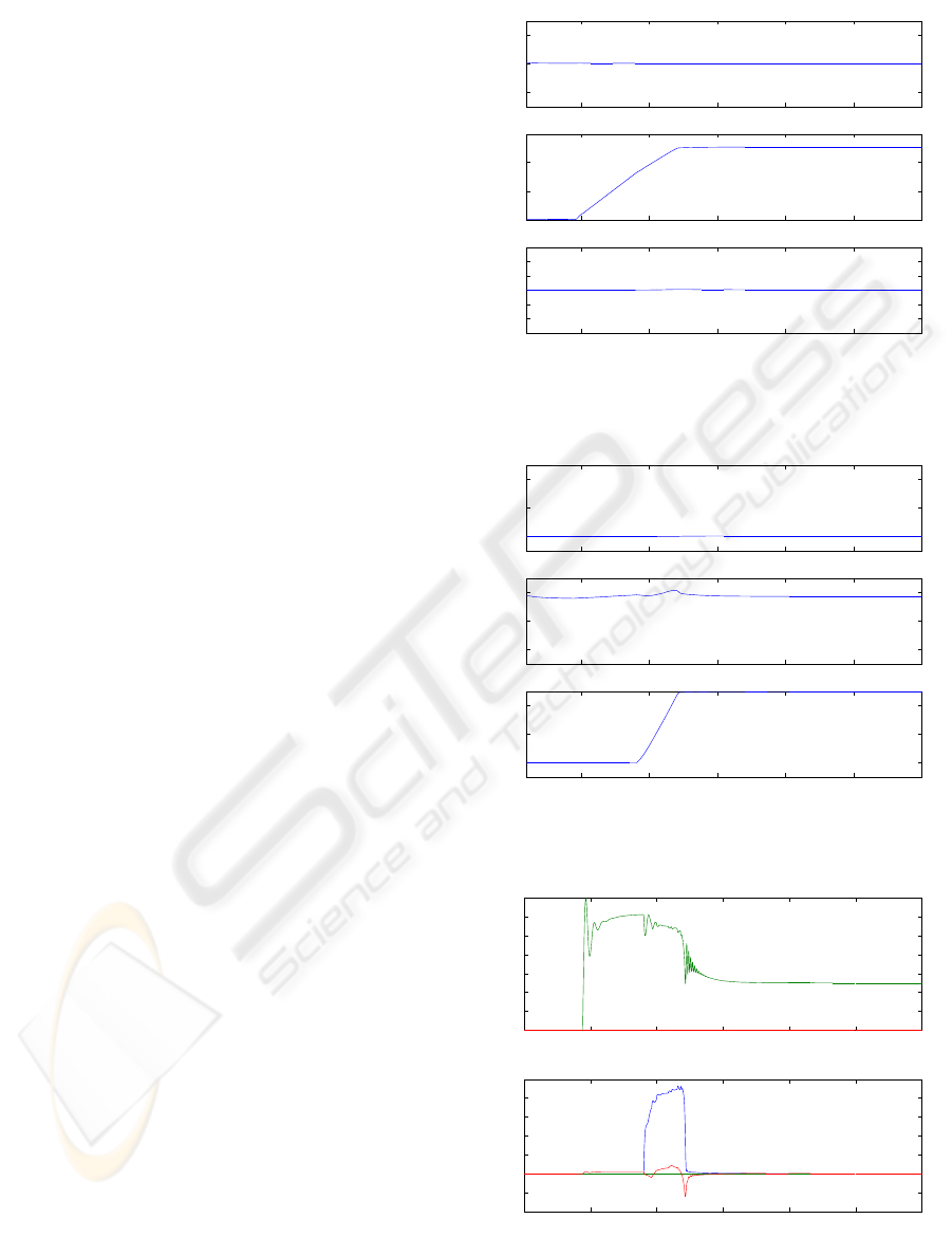
At t=0 s the manipulator is in position control, and
there is no contact between the segment and the envi-
ronment. The thrust cylinders start moving and get in
contact with the segment at t=4.8 s. The manipulator
switches to force/impedance control and moves fur-
ther with the same speed as the hydraulic thrust cylin-
ders (see Fig. 9). The y position of the environment is
at y = 0.25 m. When the segment contacts the envi-
ronment at t = 8 s, the segment aligns with the envi-
ronment as shown in Fig. 10. This contact gives rise to
a torque τ
x
of 800 Nm in the head, which is measured
by the force sensor (Fig. 11). This torque is caused by
the damping term in the impedance controller. The
rotational speed is 0.0017 rad/s the damping term is
50000, the torque is then 0.0017 × 50000 = 833 Nm.
The simulations are repeated 50 times, each time
the parameters in the controller’s internal model are
chosen randomly. In Fig. 11 and Fig. 12, the measure-
ments of the force sensor are plotted. The magnitude
of the force in the y DOF is not influenced; the time
of impact varies due to the parameter changes. The
torque around the z axis is influenced by the parame-
ter change.
4 CONCLUSIONS
A dynamic model of the manipulator and its environ-
ment has been successfully derived and implemented
in Matlab/Simulink. The control requirements have
5 10 15 20 25 30
4.2
4.3
4.4
x[m]
time(s)
Position of segment Center of Grafity
5 10 15 20 25 30
0
0.1
0.2
y[m]
time(s)
5 10 15 20 25 30
−0.1
−0.05
0
0.05
0.1
z[m]
time(s)
Figure 9: Position of the segment.
5 10 15 20 25 30
0
0.02
0.04
Roll[rad]
time(s)
Roll Pitch and Yaw angles of the segment
5 10 15 20 25 30
−0.04
−0.02
0
Pitch[rad]
time(s)
5 10 15 20 25 30
0
0.02
0.04
Yaw[rad]
time(s)
Figure 10: Orientation of the segment.
0 5 10 15 20 25 30
0
200
400
600
800
1000
1200
1400
Linear force[N]
time(s)
0 5 10 15 20 25 30
−400
−200
0
200
400
600
800
1000
Torque[Nm]
time(s)
f
y
τ
x
τ
z
Figure 11: Force measurement in the segment force sensor
(one simulation run).
HYBRID CONTROL DESIGN FOR A ROBOT MANIPULATOR IN A SHIELD TUNNELING MACHINE
191
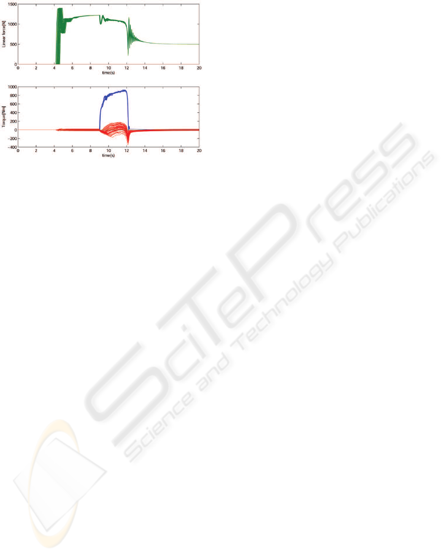
Figure 12: Force measurement in the segment force sensor
(50 simulation runs).
been met by using a combination of a force con-
troller, an impedance controller and a position con-
troller. The position precision is 0.01 m and for the
orientation the precision is 0.005 rad (0.3 degrees)
The hybrid controller is based on feedback lin-
earization to make the system linear and decoupled.
The feedback linearization is an inverse model of the
manipulator. If the dynamic parameters in the feed-
back linearization are within 10% accuracy and the
dimensional parameter are within 1% accuracy, a sta-
ble hybrid controller is obtained in simulations.
The position loops in the hybrid controller consist
of a PD-controller. The P and the D gains are tuned
by applying the following rules. When the natural fre-
quency ω and the damping ratio ζ are known, then the
P-gain is defined by ω
2
and the D-gain is defined by
2ζω.
It is assumed that the manipulator head is equipped
with a six DOF force sensor. If this is not possible
in the mechanical design, the possibility must be in-
vestigated of estimating the force, by measuring the
pressures in the hydraulic actuators.
REFERENCES
Hogan, N. (1985). Impedance control: An approach to ma-
nipulation: Part i - theory, part ii - implementation,
part iii - applications. ASME Journal of Dynamic Sys-
tems, Measurement, and Control, 107:1–24.
K. Kosuge et al. (1996). Assembly of segments for shield
tunnel excavation system using task-oriented force
control of parallel link mechanism. IEEE.
Raibert, M. and Craig, J. (1981). Hybrid position/force con-
trol of manipulators. J of Dyn Sys, Meas, and Cont.
Siciliano, B. and Villani, L. (1999). Robot Force Control.
Kluwer Academic Publishers.
Spong, M. W. and Vidyasagar, M. (1989). Robot Dynamics
and Control. John Wiley & Sons.
Tanaka, Y. (1995). Automatic segment assembly robot for
shield tunneling machine. Microcomputers in Civil
Engineering, 10:325–337.
Vukobratovi
´
c, M. (1994). Contact control concepts in ma-
nipulation robotics-an overview. In IEEE Transac-
tions on industrial electronics, vol. 41, no. 1, pages
12–24.
Zhang, H., Zhen, Z., Wei, Q., and Chang, W. (2001).
The position/ force control with self-adjusting select-
matrix for robot manipulators. In Proceedings of the
2001 IEEE International Conference on Robotics &
Automation. Department of Automatic Control, Na-
tional University of Defense Technology.
ICINCO 2004 - ROBOTICS AND AUTOMATION
192
