Spot Detection in Microscopy Images using Convolutional Neural

Network with Sliding-Window Approach

Matsilele Mabaso

, Daniel Withey

and Bhekisipho Twala

MDS(MIAS), Council for Scientific and Industrial Research, Pretoria, South Africa

Department of Electrical and Mining Engineering, University of South Africa, Pretoria, South Africa

Keywords: Microscopy Images, Convolutional Neural Network, Spot Detection.

Abstract: Robust spot detection in microscopy image analysis serves as a critical prerequisite in many biomedical

applications. Various approaches that automatically detect spots have been proposed to improve the analysis

of biological images. In this paper, we propose an approach based on Convolutional Neural Network (conv-

net) that automatically detects spots using sliding-window approach. In this framework, a supervised CNN

is trained to identify spots in image patches. Then, a sliding window is applied on testing images containing

multiple spots where each window is sent to a CNN classifier to check if it contains a spot or not. This gives

results for multiple windows which are then post-processed to remove overlaps by overlap suppression. The

proposed approach was compared to two other popular conv-nets namely, GoogleNet and AlexNet using

two types of synthetic images. The experimental results indicate that the proposed methodology provides

fast spot detection with precision, recall and F_score values that are comparable with the other state-of-the-

art pre-trained conv-nets methods. This demonstrates that, rather than training a conv-net from scratch, fine-

tuned pre-trained conv-net models can be used for the task of spot detection.

1 INTRODUCTION

Object recognition in images has been a major

research area in computer vision that arises in many

real-world applications, such as surveillance (Varga

& Szirányi, 2016), robotics (Wang, et al., 2016),

biology (Li, et al., 2014) and etc. The main goals of

this area are: Firstly, determining what kinds of

objects are present in the image (classification) and,

secondly, the location of these objects in the image

(localization). Knowing which objects are present in

a given image, computing their locations should be

easier; alternatively, knowing where to look,

recognizing the objects should be easier. In other

words, it is important to think of these two tasks

jointly. A lot of existing state-of-the-art object

classification methods does not compute the object

location information.

In this work, we focus on detection of spots in

microscopy images, as shown in Figure 1, but the

methodology can be applied in other applications.

The ability to accurately detect spots is of significant

interests for biomedical researchers as it plays a

significant step for further analysis. A Number of

procedures in biology and medicine require spot

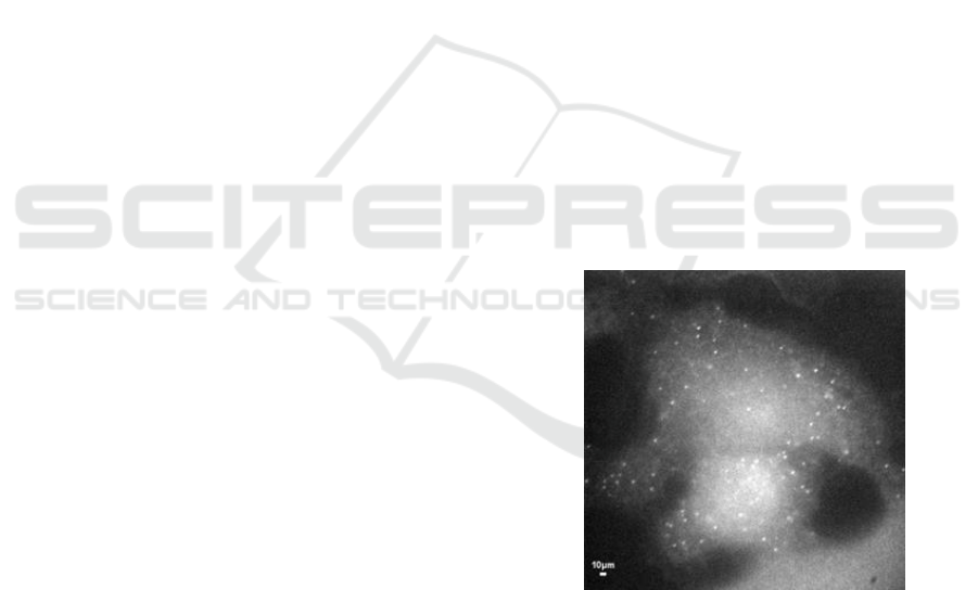
Figure 1: A sample of real fluorescence image with bright

particles obtained using confocal microscopy.

detection and counting, for example, an individual’s

health can be deduced based on the number of red

and white blood cells. Spot detection is interested in

finding all instances of spots in a given image. There

exist several challenges faced by spot detection.

Among them are noise and inhomogeneity which

exist in the background. Besides all these challenges

a lot of applications in bioimage analysis such as

spot tracking (Genovesio, et al., 2006), require high

Mabaso, M., Withey, D. and Twala, B.

Spot Detection in Microscopy Images using Convolutional Neural Network with Sliding-Window Approach.

DOI: 10.5220/0006724200670074

In Proceedings of the 11th International Joint Conference on Biomedical Engineering Systems and Technologies (BIOSTEC 2018) - Volume 2: BIOIMAGING, pages 67-74

ISBN: 978-989-758-278-3

performance and reliable detection results which

increases the need for efficiency.

Over the past years, researchers have developed

various methods for the detection of spots in

microscopy images, examples include Wavelets

(Olivo-Marin, 2002), Mathematical morphology

(Kimori, et al., 2010). A detailed review of some of

these methods can be found in (Smal, et al., 2010).

Smal et al. (Smal, et al., 2010) categorized spot

detection methods into ‘supervised’ and

‘unsupervised’ methods. Supervised methods are

machine learning methods which require ground

truth and labeled data for training. Examples of these

methods include Adaptive boosting, Fisher

discriminant analysis. Smal et al. (Smal, et al., 2010)

claimed that these techniques have better detection

performance in the image with low signal-to-noise

ratio (SNR). Unsupervised methods refer to methods

which do not require training. Recent development

in machine learning, namely deep learning has

demonstrated remarkable performance within the

task of image classification.

The convolutional neural network (conv-net) is

one of the popular and effective deep learning

techniques which based on the ImageNet

classification completion which took place 2012,

managed to bring down the error rate by half on the

classification problem. According to He et al. (He, et

al., 2015) a well-trained deep conv-net architecture

can famously perform better than humans in

identifying objects in images. The conv-nets have

since been adopted to various applications in

computer vision community (Noh, et al., 2015) and

medical image analysis (Tajbakhsh, et al., 2016).

Several different conv-nets architectures have since

been developed since 2012, AlexNet (Krizhevsky, et

al., 2012), VGGNet (Simonyan & Zisserman, 2014),

ResNet (He, et al., 2015) and GoogLeNet (Szegedy,

et al., 2015) among others. Despite the range of

their applications in different fields, conv-nets have

only introduced lately to analyze biological data, and

recent works indicate that conv-nets have significant

potential in addressing the needs of a biologist in

analyzing data (Van Valen, et al., 2016).

To our knowledge, there exist no conv-net

architecture for the detection of spots in microscopy

images. As such this work introduces an approach

for the detection of spots based on conv-net and a

sliding window approach. The sliding window is

based on the idea of sliding a box around an image

and classify each image crop inside a box (contains a

spot or not).

This paper is organized as follows: Section 2

describes the methodology used in the study, while

Section 3 presents the results and finally, Section 4

concludes the paper.

2 MATERIAL AND METHOD

2.1 Methodology

2.1.1 Convolutional Neural Network

(Conv-Net)

A convolutional neural network (conv-net)  is a

composition of sequence of  layers (



……



) that

maps an input vector  to an output vector , i.e.,

  













 





































 











(1)

where 



is the weight and bias vector for the 



layer 



and 



is determined to perform one of the

following: a) convolution with a bank of kernels; b)

spatial pooling; and c) non-linear activation. For any

given  training datasets 



















, we can

estimate the weights, 







by solving the

optimization problem:







































(2)

Where  is defined as the loss function. The

numerical optimization of equation (2) is often

performed via backpropagation and stochastic

gradient descent methods (Ruder, 2017).

2.1.2 Problem Formulation

Given a set of labeled training images, grayscale

image patches defined as 



 



, for  in range

1 to  with dimensionality      for each

image patch. The idea is to train a conv-net to

predict if patch, 



contains a spot or not. Image

patches with a full spot contained in the image are

labelled as positive, otherwise negative.

2.1.3 Proposed Convnet

Generally, conv-nets include some of the following

types of layers:

a) Convolution layers, these layers are the

basis of the conv-net architecture and

perform the main computations of the

network including training and firing of

BIOIMAGING 2018 - 5th International Conference on Bioimaging

neurons. They work by convolving a kernel

of given size across an input image and

compute the response function over at each

location of the filter.

b) Pooling or down-sampling layers. These

layers are usually put after each conv layer

and reduce the size of the input image for

the next conv layer. It works by sliding a

window and takes the maximum value from

the values within a window at a given

location.

c) Fully connected layers: These layers have

all connection from all neurons in the

previous layer to all output. The main

purpose of the fully connected layer is to

use features form convolutional and

pooling layers for classification of the input

image to various classes. They are typically

used as the last layer in a conv-net, with the

output having one element per class label.

Given the above building blocks, we propose conv-

net architecture for spot detection, named detectSpot

as shown in Table 1. The proposed conv-net consists

of 5 layers (3 convolution layers and 2 fully

connected layers) with learnable weights. We

employ a Rectified Liner Unit (ReLu) (Nair &

Hinton, 2010) activation function for the first four

layers and a softmax for the last layer.

We apply dropout with probability of 0.5 for the

first two fully connected layers (FC). The weights

were initialized using truncated random normal.

Cross-entropy loss was minimized using Adam

optimization with the initial learning rate of 0.001.

Table 1: Proposed conv-net architecture.

Layer

Kernel size,

stride

Output

    

Input

Conv

ReLu

Max-Pool



  

  

    

    

    

Conv

ReLU

Max-Pool

  

  

    

    

Conv

ReLu

Max-Pool

  

  

    

    

ReLu+Dropout





ReLu+Dropout





Softmax





2.1.4 Sliding-Window

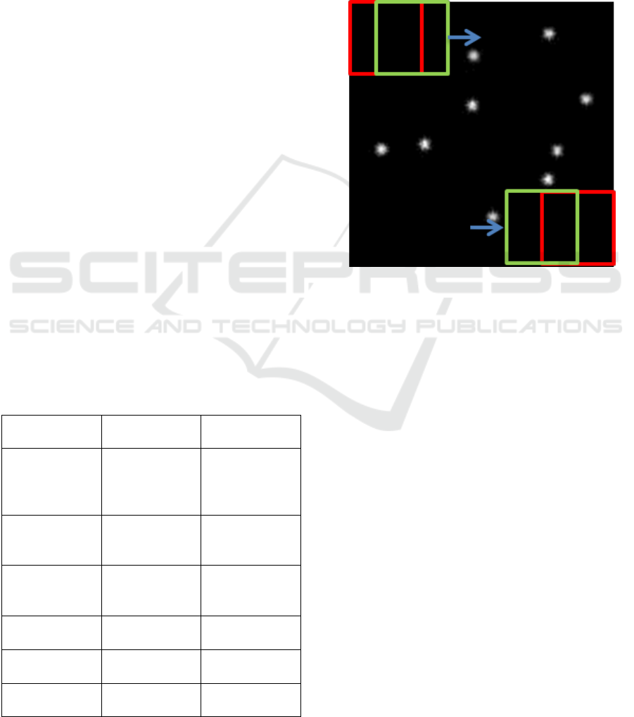
The procedure adopted for detecting all spots

positions in an image is based on sliding-window

technique. Sliding-window is a technique of sliding

a rectangular window across an image from top to

bottom and left to right as illustrated by red and

green rectangles in Figure 2. This is done in order to

analyze subpart of the image and extract some

information.

Figure 2: Illustration of sliding-window approach.

2.1.5 Dataset

Synthetic image patches sampled from a synthetic

image of size    were used for training a

proposed conv-net. Each image patch was of size

   pixels. Positive patches were identified as

those which contain a center of a spot and negative

patches are those which do not contain a spot. We

noted that the number of negative patches is usually

disproportionally large compared to the number of

positive patches. This was caused by the fact that

most of each image does not contain spots. Two

measures were then proposed to make training and

validation set more balanced. Firstly, we randomly

discarded negative patches so that the is 50* the

number of positive patches. Secondly, we rotated

each positive patch giving 4 extra positive patches.

A total of 21300 patches created from images with a

signal to noise ratio (SNR) of (20, 10, 5, 2, 1). A

total of 21300 The 21300 image patches were

divided as follows:

• 80% for training

• 20% evaluation

Spot Detection in Microscopy Images using Convolutional Neural Network with Sliding-Window Approach

2.1.6 Implementation and Training

To implement and tune a proposed conv-net we used

TFLearn (Damien, 2016). TFLearn is a tensorflow

(Abadi, et al., 2015) wrapper which allows simple

implementation and training of deep learning

models. The network was learned using Adam

(Kingma & Ba, 2015) based optimization algorithm.

Training was carried out on a Linux machine with

16GB RAM and Nvidia GTX680 running TFLearn

(v0.3) and tensorflow (v1.3.0) with.

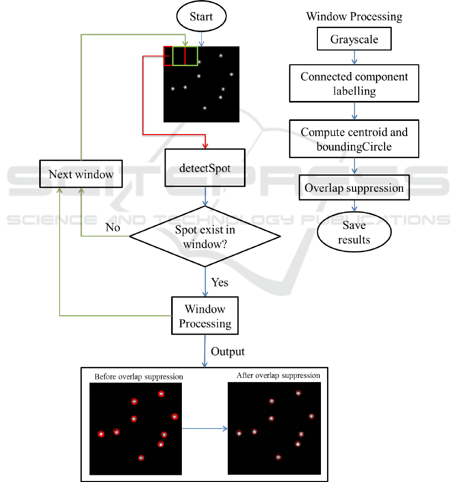
2.2 Detection of Spots in Test Images

Once the proposed conv-net architecture, deepSpot

is trained it is able to classify an image patch as

containing a spot or not. Figure 3 illustrates the

entire pipeline for the detection of spots. In order to

detect all spots in a complete image, we scan

through an image using a window of size



  



which is then passed onto a deepSpot and select

those with the highest probability of containing

spot. At each iteration, the extracted sub-window is

Figure 3: The proposed architecture for spot detection in microscopy images.

BIOIMAGING 2018 - 5th International Conference on Bioimaging

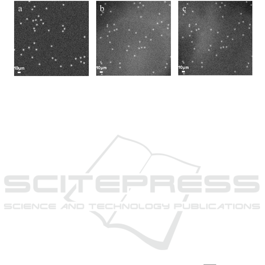
Figure 4: Examples of synthetic images used for testing with approximately 50 spots per image. (a) Type A, and (b-c)

Type B.

passed onto a classifier to compute a score S, which

defines whether a spot is contained in the sub-

window. Then, if S is bigger than the set threshold T,

the correspond-ding sub-window is considered to

contain spot.

Then, the sub-windows classified as containing

spots are subject to further processing to get spot

centroid







and bounding circles indicating the

location of spots in an image. There are two main

important parameters for our proposed sliding-

window approach, window-size



  



and stride.

These parameters influence both speed and detection

rate. This approach can only detect spots with fixed

size but it can be extended to spots with different

sizes by introducing image pyramids.

Using a small stride, e.g. stride = 1, will result in

multiple detections of the same spot at slightly

different positions. To overcome this issue, we

group all nearby detections so that every spot is

detected once by using overlap suppression (OS)

approach. The OS method works by grouping all

overlapping detections and suppresses the ones with

lowest scores. This will result in discarding all

overlapping detections.

2.2.1 Using Pre-trained Models

2.2.1.1 Pre-trained Models

The proposed detectSpot model was compared to

two other state-of-the-art conv-nets models, namely,

AlexNet and GoogleNet.

AlexNet: This conv-net was developed by

Krizhevsky et al. (Krizhevsky, et al., 2012) and

successfully applied to large-scale image recognition

and won the ImageNet ILSVRC-2012 challenge.

The model consisted of 8 layers (5 convolutional

layers and three fully connected layers).

GoogleNet: This conv-net was a winner for

ImageNet ILSVRC-2014 proposed by Szegedy et al.

(Szegedy, et al., 2015) from Google. This network

has 12X fewer parameters compared to AlexNet yet

deeper (22 layers). The main contribution of

GoogleNet is the introduction of inception module.

2.3 Synthetic Datasets and Evaluation

Criteria

2.3.1 Synthetic Test Datasets

We generated two types of synthetic datasets (Type

A and Type B) containing spots using a framework

proposed in (Mabaso, et al., 2016) in order to

demonstrate the effectiveness of the proposed

detectSpot model as shown in Figure 4. Each

synthetic image contains 50 spots cluttered on the

background of size    pixels. The dataset

was corrupted by white noise. The following signal

to noise ratios (SNR) levels was explored {10, 8, 6,

4, 2, 1} where the spot intensity was 20 gray levels.

The signal to noise ratio is defined as of spot

intensity, 



, divided by the noise standard

deviation, 



 









(1)

The spot positions were randomized using Icy-

plugin (Chenouard, 2015) to mimic the kinds of

properties in real microscopy images. MATLAB

was used to add spots and the OMERO.matlab-5.2.6

toolbox (Anon., 2016) was used to read and save

images.

2.3.2 Evaluation Criteria

Three state-of-the-art architecture The criteria used

for evaluation is based on computing Precision and

Recall. TP, FP, and FN. The precision, recall, and

 is three important measures which are

reported in machine learning research in determining

Spot Detection in Microscopy Images using Convolutional Neural Network with Sliding-Window Approach

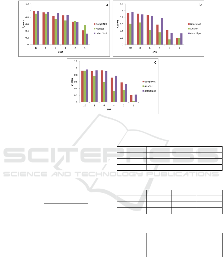
Figure 5: F_score vs SNR curves for all three conv-nets methods applied to two kinds of synthetic images (a) Synthetic

type A, and (b-c) Synthetic type B.

the performance of the classifier. Precision and

recall are defined in terms of a number of true

positives (TP), false positives (FP) and false

negatives (FN):

 



  

(relevant spots detected)

(3)

 



  

(spots detected) (4)

   

  



  



(5)

A good detection method should have the value of





approaching one.

3 RESULTS

The trained conv-nets models were each applied to

two types of synthetic images described in Section

2.3.1 as shown in Figure 4 with a signal-to-noise

ratio (SNR) in range {10, 8, 6, 4, 2, 1}. Table 2 -

Table 4 indicates the results for all three conv-nets,

detectSpot, GoogleNet and AlexNet for each of the

test sets. The results were averaged for all SNR’s.

The performance of each method measured using

precision, recall, and F_score. The fair comparison

was achieved by re-training three other conv-nets on

the same datasets. Table 2 indicates that in terms of

Table 2: Evaluation metrics calculated on sythetic images

for three classifiers.

Model

Precision

Recall



GoogleNet

0.833

0.751

0.784

AlexNet

0.842

0.703

0.758

detectSpot

0.836

0.740

0.782

Table 3: Evaluation metrics calculated on realistic

synthetic data. Background 1.

Method

Precision

Recall



GoogleNet

0.717

0.585

0.633

AlexNet

0.443

0.365

0.397

detectSpot

0.803

0.614

0.675

Table 4: Evaluation metrics calculated on realistic

synthetic data. Background 2.

Model

Precision

Recall



GoogleNet

0.733

0.699

0.708

AlexNet

0.567

0.476

0.502

detectSpot

0.780

0.675

0.721

average values, the difference in

performance for GoogleNet and deepSpot is small

compared to AlexNet method. The recall rates are

higher for GoogleNet in Table 2 and Table 4. This

indicates that the method was able to correctly detect

true spots compared to other methods while AlexNet

method has a higher precision. Higher precision

indicate that the method detected less false spots in

comparison to others. However, it shows in Table 3

BIOIMAGING 2018 - 5th International Conference on Bioimaging

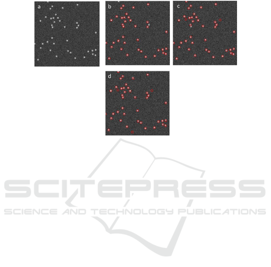
Figure 6: Results of applying the proposed conv-nets methods on a synthetic image data. Detected spots by each method

are showed in red circles.(a) Original synthetic image. (b) Spots detected by our approach, detectSpot. (c) Detected spots

using using GoogleNet. (d) Detected spots with AlexNet.

and Table 4 that GoogleNet and AlexNet reported

low values for precision compared to detectSpot.

Fig. 5 shows the behavior of each method at all

different signal-to-noise ratios. It can be noted from

the figure that the performance of GoogleNet and

detectSpot is comparable similar for Fig. 5 (a) at

SNR = 10, 8, 2, 4 while AlexNet has higher

 at SNR = 1 on Type A images and drops

on Type B images. In Type B synthetic images as

shown in Figure 5(b-c) it indicates that has slightly

higher values for all SNRs. However, the difference

in performance of detectSpot and GoogleNet is

relatively small.

Figure 6 illustrate the performance of each

method on Type A synthetic images with SNR = 10.

4 CONCLUSIONS

Spot detection is an important step towards the

analysis of microscopy images. Over the years,

different approaches have been developed that on

segmentation to perform spot detection.

In this study, we have presented an automated

approach for the detection and counting of spots in

microscopy images, termed detectSpot. The

proposed approach is based on a convolutional

neural network with a sliding-window based

approach to detect multiple spots in images. The

comparative experiments demonstrated that the

GoogleNet and detectSpot methods achieved

comparable performance compared to the AlexNet

method. We also have shown that rather training a

convnet from scratch, knowledge transfer from

natural images to microscopy images is possible. A

fine-tuned pre-trained conv-net can give results

which are comparable to fully trained conv-net.

ACKNOWLEDGEMENTS

This work was carried out in financial support from

the Council for Scientific and Industrial Research

(CSIR) and the Electrical and Electronic

Engineering Department at the University of

Johannesburg.

REFERENCES

Abadi, M. et al., 2015. TensorFlow: Large-scale machine

learning on heterogeneous systems. s.l.:12th USENIX

Symposium on Operating Systems Design and

Implementation.

Anon., 2016. The open microscopy environment. [Online]

Available at: http://www.openmicroscopy.org/site/

support/omero5.2/developers/Matlab.html [Accessed

15 November 2016].

Chenouard, N., 2015. Particle tracking benchmark

generator. [Online] Available at: http://icy.bioimage

Spot Detection in Microscopy Images using Convolutional Neural Network with Sliding-Window Approach

analysis.org/plugin/Particle_tracking_benchmark_gen

erator [Accessed 1 November 2016].

Damien, A., 2016. TFLearn. s.l.:GitHub.

Genovesio, A. et al., 2006. Multiple particle tracking in

3d+t microscopy: Method and application to the

tracking of endocytosed quantum dots. IEEE Trans.

Image Process., 15(5), pp. 1062-1070.

He, K., Zhang, X., Ren, S. & Sun, J., 2015. Deep residual

learning for image recognition. s.l., s.n.

He, K., Zhang, X., Ren, S. & Sun, J., 2015. Deep residual

learning for image recognition. s.l., s.n., pp. 770-778.

Kimori, Y., Baba, N. & Morone, N., 2010. Extended

morphological processing: a practical method for

automatic spot detection of biological markers from

microscopic images. BMC Bioinformatics, 11(373),

pp. 1-13.

Kingma, D. P. & Ba, J. L., 2015. Adam: A method for

stochastic optimization. San Diego, s.n.

Krizhevsky, A., Sutskever, I. & Hinton, G. E., 2012.

Imagenet classication with deep convolutional neural

networks. s.l., s.n., pp. 1-9.

Li, R. et al., 2014. Deep learning based imaging data

completion for improved brain disease diagnosis.

Quebec City, s.n.

Mabaso, M., Withey, D. & Twala, B., 2016. A framework

for creating realistic synthetic fluorescence

microscopy image sequences. Rome, s.n.

Nair, V. & Hinton, G. E., 2010. Rectified Linear Units

Improve Restricted Boltzmann Machines. s.l., s.n., pp.

807-814.

Noh, H., Hong, S. & Han, B., 2015. Learning deconvolu-

tion network for semantic segmentation. s.l., s.n.

Olivo-Marin, J.-C., 2002. Extraction of spots in biological

images using multiscale products. Pattern

Recognition, 35(9), pp. 1989-1996.

Ruder, S., 2017. An overview of gradient descent

optimization algorithms. [Online] Available at:

http://ruder.io/optimizing-gradient-descent/[Accessed

10 October 2017].

Simonyan, K. & Zisserman, A., 2014. Very deep

convolutional networks for large-scale image

recognition. s.l., s.n.

Smal, I., Loog, M., Niessen, W. & Meijering, E., 2010.

Quantitative comparison of spot detection methods in

fluorescence microscopy. IEEE Trans on Medical

Imaging, 29(2), pp. 282-301.

Szegedy, C. et al., 2015. Going Deeper with Convolutions.

Boston, s.n.

Tajbakhsh, N. et al., 2016. Convolutional Neural

Networks for Medical Image Analysis: Full Training

or Fine Tuning?. IEEE Transactions on Medical

Imaging, May, 35(5), pp. 1299-1312.

Van Valen, D. A. et al., 2016. Deep learning automates the

quantitative analysis of individual cells in live-cell

imaging experiments. PLoS Comput Biol, November,

12(11), pp. 1-24.

Varga, D. & Szirányi, T., 2016. Detecting pedestrians in

surveillance videos based on convolutional neural

network and motion. Budapest, Hungary, s.n., pp.

2161-2165.

Wang, Z., Li, Z., Wang, B. & Liu, H., 2016. Robot grasp

detection using multimodal deep convolutional neural

networks. Advances in Mechanical Engineering,

August, 8(9), pp. 1-12.

BIOIMAGING 2018 - 5th International Conference on Bioimaging