
The Mapping Distance – a Generalization of the Edit Distance – and its
Application to Trees
Kilho Shin
1
and Taro Niiyama
2
1
University of Hyogo, Kobe, Japan
2
NTT DoCoMo, Tokyo, Japan
Keywords:
Edit Distance, Kernel, Mapping, Tree.
Abstract:
The edit distances has been widely used as an effective method to analyze similarity of compound data, which
consist of multiple components, such as strings, trees and graphs. For example, the Levenshtein distance for
strings is known to be effective to analyze DNA and proteins, and the Ta
¨
ı distance and its variations are at-
tracting wide attention of researchers who study tree-type data such as glycan, HTML-DOM-trees, parse trees
of natural language processing and so on. The problem that we recognize here is that the way of engineering
new edit distances was ad-hoc and lacked a unified view. To solve the problem, we introduce the concept
of the mapping distance. The mapping distance framework can provide a unified view over various distance
measures for compound data focusing on partial one-to-one mappings between data. These partial one-to-one
mappings are a generalization of what are known as traces in the legacy study of edit distances. This is a clear
contrast to the legacy edit distance framework, which define distances between compound data through edit
operations and edit paths. Our framework enables us to design new distance measures consistently, and also,
various distance measures can be described using a small number of parameters. In fact, in this paper, we
take rooted trees as an example and introduce three independent dimensions to parameterize mapping distance
measures. As a result, we define 16 mapping distance measures, 13 of which are novel. In experiments, we
discover that some novel measures outperform the others including the legacy edit distances in accuracy when
used with the k-NN classifier.
1 INTRODUCTION
Edit distances have proven to be effective to measure
similarity of compound data such as strings, trees and
graphs. By a compound datum, we mean a datum that
consists of one or more components: a string consists
of letters, and a tree and a graph consist of vertices
and edges.
The Levenshtein distance for strings (Levensh-
tein, 1966) is a well-known example of edit distance
measures. Ta
¨
ı extended the Levenshtein distance to
trees and introduced the first instance of edit distance
measures that measure similarity between trees (Ta
¨
ı,
1979). Since computing Ta
¨
ı distances requires he-
avy computation, a number of its variations have been
proposed in the literature including the constrained
distance (Zhang, 1995), the less-constrained distance
(Lu et al., 2001) and the degree-two distances (Zhang
et al., 1996). Their definitions are all stemmed from
the Ta
¨
ı distance, and they have succeeded in reducing
computational complexity of the Ta
¨
ı distance. On the
other hand, Wang and Zhang (Wang and Zhang, 2001)
introduced the alignment distance to extend the con-
cept of string alignments to trees. In fact, the align-
ment distance has turned out to be identical to the less
constrained distance (Kuboyama et al., 2005). For
graphs, a definition of edit distances is given in (Neu-
haus and Bunke, 2007).
When we survey the study history of the tree edit
distance, we see that many different definitions have
been introduced in the literature, but the ways to in-
troduce them appeared ad-hoc rather than being ame-
nable to discipline. Therefore, we cannot deny the
possibility that we have missed instances of the edit
distance measure that have good performance in accu-
racy or time-efficiency or both.
Two of the important contributions of this paper
are to introduce the notion of the mapping distance,
which generalizes the legacy edit distance with a con-
sistent view, and to engineer new distance measures
for trees through three novel parameters obtained by
leveraging the mapping distance framework.
In the following sections, we introduce the notion
of mapping distances and clarify their advantages. To
266
Shin, K. and Niiyama, T.
The Mapping Distance – a Generalization of the Edit Distance – and its Application to Trees.
DOI: 10.5220/0006721902660275
In Proceedings of the 10th International Conference on Agents and Artificial Intelligence (ICAART 2018) - Volume 2, pages 266-275
ISBN: 978-989-758-275-2
Copyright © 2018 by SCITEPRESS – Science and Technology Publications, Lda. All rights reserved

illustrate, we develop our discussion focusing on ap-
plication to trees. In fact, we introduce 16 instances of
mapping distance measures for trees. Although three
of them are well-known in the literature, the remain-
der are novel and are not investigated in the literature.
In addition, we report the results of experiments that
we run to compare these mapping distance measures.
As a result, we have discovered that the distance me-
asures that exhibit the best accuracy performance are
novel measures.
2 LEGACY EDIT DISTANCES
FOR TREES
Just for convenience of explanation, we mean rooted
trees by “trees”. Therefore, in this paper, a tree has
always a root vertex, and all of the other vertices are
its descendants.
In the traditional way, edit distances are defined
based on edit operations, edit paths and edit costs. To
illustrate, we let X and Y be two trees. An edit path
from X to Y is a sequence of edit operations, which is
one of (1) to substitute a vertex y of Y for a vertex x
of X (denoted by (x, y)); (2) to delete a vertex x of X
(denoted by (x, ⊥)); the children of x is re-defined as
children of the parent of x; (3) to insert a vertex y of Y
below a vertex in the relevant tree as a child (denoted
by (⊥, y)); an arbitrary subset of the child vertices of
the vertex below which y is inserted can be selected
and re-defined as child vertices of y.
Example 1. Fig. 1 exemplifies an edit path for the Ta
¨
ı
distance. The leftmost tree is X , while the rightmost
tree is Y. We first delete the vertex x
b
(the vertex with
label “b”) from X. The children of x
b
is re-defined as
children of the root x
a
. Next, we substitute the ver-
tices y
a
, y
c
, y
d
and y
g
of Y for the vertices x
a
, x
c
, x
d
and x
e
, and obtain X
2
. Finally, we insert the vertex y
f
below the root y
a
of X
2
. To determine children of the
new vertex y
f
, we select y
d
and y
g
. Hence, the edit
path here is represented by
(x
b
,⊥)(x
a
,y
a
)(x
c
,y
c
)(x
d
,y
d
)(x
e
,y
g
)(⊥,y
f
).
a
b
ec
d
X
1
= X
a
c
d
g
X
2
a
c
f
d
g
X
3
= Y
Figure 1: An edit path and a trace (dotted arrows) of the Ta
¨
ı
distance: (x
b
,⊥)(x
a
,y
a
)(x
c
,y
c
)(x
d
,y
d
)(x
e
,y
g
)(⊥,y
f
).
To each edit operation is assigned a cost, which
is usually a non-negative real number. We let γ(v,w),
γ(v,⊥) and γ(⊥,w) denote the costs of substituting w
for v, deleting v and inserting w. When `(v) denotes
the label of a vertex v, the most common setting of
costs is:
γ(v,w) =
(
0, if `(v) = `(w);
1, if `(v) 6= `(w).
γ(v,⊥) = γ(⊥, w) = 1. (1)
Then, the cost of an edit path is the sum of the costs
of the operations that comprise the path: for example,
the cost of the path of Fig. 1 is 3. The Ta
¨
ı distance
d
T
(X,Y ) is the minimum cost across all possible edit
paths from X to Y (Ta
¨
ı, 1979).
Many variations of the Ta
¨
ı distance are known in
the literature. The degree-two distance (Zhang et al.,
1996) is an example and poses the constraint that only
vertices with degree one and two can be deleted and
inserted. The degree of a vertex is the number of ed-
ges that the vertex has, and the degree-two distance is
the minimum cost of edit paths under this constraint.
a
b
ec
d
X
1
= X
a
c
f
g
X
2
a
c
f
d
g
X
3
= Y
Figure 2: An edit path and a trace of the degree-two dis-
tance: (x
d
,⊥)(x
b
,⊥)(⊥,y
f
)(x
a
,y
a
)(x
c
,y
c
)(x
e
,y
g
)(⊥,y
d
).
Example 2. In Fig. 2, the vertex x
d
is of degree one,
and hence, we can delete it. The degree of x
b
has
changed from three to two after deleting x
d
, we can
delete it. On the other hand, we can insert y
f
between
x
a
and x
c
, because its degree is two. In the same way
as Example 1, we substitute the vertices y
a
, y
c
and y
g
of Y for the vertices x
a
, x
c
and x
e
. Then, we obtain
X
2
. Finally, we insert y
d
, whose degree is one. The
corresponding edit script is
(x
d
,⊥)(x
b
,⊥)(⊥,y
f
)(x
a
,y
a
)(x
c
,y
c
)(x
e
,y
g
)(⊥,y
d
),
and its cost is five.
The trace of an edit path is a partial one-to-one
mapping between the vertex sets of X and Y , deter-
mined by the substitution operations included in the
path. For the edit path of Example 1, the trace deter-
mines (x
a
→ y
a
,x
c
→ y
c
,x
d
→ y
d
,x
e
→ y
g
), while that
of Example 2 does (x
a
→ y
a
,x
c
→ y
c
,x
e
→ y
g
). The
domain and the range of a trace τ are those of τ as a
partial mapping. For example, when we denote the
trace of Example 1 by τ, the domain Dom(τ) and the
range Ran(τ) are {x
a
,x
c
,x
d
,x
e
} and {y
a
,y
c
,y
d
,y
g
},
respectively.
The constrained distance (Zhang, 1995), on the ot-
her hand, poses a constrain on traces.
The Mapping Distance – a Generalization of the Edit Distance – and its Application to Trees
267

In the remainder of this paper, we denote the nea-
rest common ancestor (NCA) of vertices v and w in a
tree X by v ` w. More generally, for a set S of vertices
of X, S
`
denotes the nearest common ancestor of all
of the vertices of S.
Definition 1. Two sets S and T of vertices are separa-
ble, iff S
`
and T
`
are not in the ancestor-descendent
relation.
Definition 2 . A trace τ of an edit path is said to be
separable, when S ⊆ Dom(τ) and T ⊆ Dom(τ) are
separable in X, iff τ(S) and τ(T ) are separable in Y .
The constrained distance requires that traces are
always separable and is the minimum cost of edit
paths under this constraint.
Example 3 . The trace of the edit path of Exam-
ple 1 is not separable. In fact, we let S = {x
c
,x
d
}
and T = {x
e
}. Since S
`
= x
b
and T
`
= x
e
, S and T
are separable in X . By contrast, τ(S)
`
= y
a
is the root
of Y , and hence, τ(S) and τ(T ) are not separable.
3 MAPPING DISTANCES
The conditions that determine the edit paths of the Ta
¨
ı
and degree-two distances can be equivalently descri-
bed as constraints on their associated traces. To be
specific, an edit path complies to the Ta
¨
ı or degree-
two distance, if, and only if, its associated trace meets
the following condition.
Ta
¨
ı: A trace preserves the relation of ancestors and
descendants: x
1
is an ancestor of x
2
in Dom(τ) ⊆
X, iff τ(x
1
) is an ancestor of τ(x
2
) in Y .
Degree-two: A trace preserves the relation of NCA:
if x
1
and x
2
are in Dom(τ) ⊆ X, then x
1
` x
2
∈
Dom(τ) and τ(x
1
` x
2
) = τ(x
1
) ` τ(x
2
) hold.
These constraints on traces require that traces as
mappings preserve particular intrinsic structures of
trees.
Ta
¨
ı: If a vertex v is an ancestor of a vertex w in a tree
X, we denote v > w. This makes X a partial orde-
red set (poset). Hence, the condition stated above
requires v > w ⇔ τ(v) > τ(w). In other words, τ
and τ
−1
are homomorphisms of posets.
Degree-two: A tree X can be defined as an
algebraic structure (X, `) so that v
`
v = v,
v
`
w = w
`
v,(v
`
w)
`
u = v
`
(w
`
u) and v
`
w
`
u ∈
{v
`
w,w
`
u,u
`
v} hold for any {v,w,u} ⊆ X. The
condition stated above means that τ and τ
−1
are
homomorphisms, that is, τ(v
`
w) = τ(v)
`
τ(w)
holds for any {v, w} ⊆ Dom(τ) ⊆ X.
On the other hand, given an edit path π and the
associated trace τ, the cost γ(π) is calculated by
γ(π) =
∑
v∈X\Dom(τ)
γ(v,⊥) +
∑
w∈X\Ran(τ)
γ(⊥,w) +
∑
v∈Dom(τ)
γ(v,τ(v)).
Since the left-hand side is a function of τ, we also
denote it by γ(τ).
To determine a mapping distance d(X,Y ) between
X and Y , we first determine a set M
X,Y
per pair (X,Y )
that consists of partial one-to-one mappings from X
to Y , and then, we let d(X,Y ) = min
µ∈M
X,Y
γ(µ).
Furthermore, we let X be a set of trees for which
distances are to be computed and assume that a set
of mapping M
X,Y
is uniquely assigned to each pair
(X,Y ) ∈ M
2
. By requiring µ ∈ M
X,Y
⇒ µ
−1
∈ M
Y,X
and symmetry of the cost function γ, that is, γ(v, w) =
γ(w,v) and γ(v,⊥) = γ(⊥, v), the resulting distance
measure has symmetry. Hence, d(X,Y ) = d(Y,X)
holds. Regarding the triangle inequality d(X,Y ) +
d(Y, Z) ≥ d(X , Z), we have the following theorem.
Theorem 1 . If a family of sets of partial mappings
M = {M
X,Y
| (X,Y ) ∈ X
2
} is transitive, that is, if
µ ∈ M
X,Y
and ν ∈ M
Y,Z
, ν ◦ µ ∈ M
X,Z
, the triangle in-
equality holds for the resulting mapping distance.
4 PARAMETERIZING TRACES
The framework of the mapping distance also suits
parameterizing mapping distance measures. In this
section, we introduce a set of parameters that describe
a certain class of mapping distances for trees. Once
such parameters are given, by testing all of the combi-
nations of parameter values, we can find the distance
measure that fits to the relevant application the best.
For simplicity, we pose two premises on the partial
mappings (traces) to investigate.
• We focus on rooted trees: the relation of ancestor
and descendants is given among vertices.
• Traces preserve the relation of ancestors and des-
cendants: v > w ⇔ τ(v) > τ(w) always holds.
The parameters we introduce below are shape
type, inter-vertex gap and exact label match.
4.1 Shape Type
This parameter determines domains and ranges of
traces. In this paper, we determine five possible
values for this parameter, namely, Forest, Tree,
Agreement, Path and Separable.
Forest: This value specifies that Dom(τ) and Ran(τ)
can be arbitrary subsets of trees X and Y , and
ICAART 2018 - 10th International Conference on Agents and Artificial Intelligence
268

τ does not require anything more than that τ is
a homomorphism of posets with respect to the
ancestor-descendent order. This value applies to
the Ta
¨
ı edit distance.
Tree: This value specifies that Dom(τ) and Ran(τ)
have the maximum vertices with respect to the
ancestor-descendent relation, and τ does not re-
quire anything more than that τ is a homomor-
phism of posets with respect to the ancestor-
descendent order.
Agreement: This value specifies that Dom(τ) and
Ran(τ) are closed under the NCA operation, and
τ is a homomorphism of algebraic structures with
respect to the NCA operator. This value applies to
the degree-two edit distance.
Path: This value specifies that Dom(τ) and Ran(τ)
are totally ordered sets with respect to the
ancestor-descendent relation, and τ is a homomor-
phism of posets.
Separable: Definition 2 defines this value. Dom(τ)
and Ran(τ) can be arbitrary subsets of trees X and
Y , and τ is separable. This value applies to the
constrained edit distance.
4.2 Inter-vertex Gap
The parse-tree kernel (Collins and Duffy, 2001)
counts the number of so-called co-rooted subtrees
shared between two trees. The basic idea of the ker-
nel is that, the more co-rooted subtrees the trees share,
the more similar are the trees. What we should note
here is that a co-rooted subtree does not allow gaps
between their vertices: If two vertices are in the re-
lation of parent and child in a co-rooted subtree, they
are also a parent and a child in the original tree.
Gaps are not allowed, Gaps are allowed.
Figure 3: Inter-vertex gaps: vertices in gray determines a
subtree.
By contrast, the distances that we saw in Section 1
all allow gaps. Hence, the second parameter inter-
vertex gap determines whether Dom(τ) and Ran(τ)
allow gaps between their adjacent vertices.
4.3 Exact Label Match
In (Shin, 2015), a method to convert edit distance pro-
blems into pattern extraction problems is shown. In
particular, the author of the paper has derived Mos-
tly Adjusted Agreement Sub-Tree (MAAST) problem
from the degree-two distance, which relaxes the con-
straint of exact match of labels of the well-known
MAST problem (Kao et al., 2007).
First, we briefly review MAST problem. To make
the explanation simple, we take two rooted trees
X
1
and X
2
and consider agreement subtrees between
them. In Fig. 4, Y is an agreement subtree with em-
beddings ε
1
: Y → X
1
and ε
2
: Y → X
2
. The embed-
dings are required to preserve the relation of ancestors
and descendants, the NCA relation and vertex labels.
The MAST problem is a problem to find the largest
agreement subtree in size. In other words, the ob-
jective function of optimization is the size |Y |.
a
b
ec
d
X
1
a
c e
Y
a
c
f
d
e
X
3
ε
1
ε
2
Figure 4: An agreement subtree and the MAST problem.
On the other hand, Fig. 5 depicts a trace τ of the
edit path of Fig. 2. Actually, ε
2
◦ ε
−1
1
is comparable
with τ, and the only difference is that τ does not ne-
cessarily preserve labels of vertices. In fact, in Fig. 5,
τ maps the vertex labeled “e” of X
1
to the vertex labe-
led “g” of X
2
.
a
b
e
c
d
X
1
a
c
f
d
g
X
3
τ
Figure 5: A trace of the degree-two distance.
In (Shin, 2015), a non-negative penalty function p
is introduced, and the MAAST problem is defined as
a problem to maximize the objective function of the
form of |Dom(τ)| − p(τ). p(τ) = 0, iff τ preserves
vertex labels.
The author has also proven that the τ that maximi-
zes this objective function also yields the degree-two
distance.
The significance of (Shin, 2015) consists in defi-
ning a new type of pattern extraction problems relax-
ing the constraint of the exact label match and having
shown the equivalence between solving the MAAST
problem and computing the degree-two distance.
Reversely, this inspires us to introduce a new class
of edit distances by requiring exact label match for
traces. Thus, the last parameter that we introduce de-
termines whether or not exact label match is required
for traces.
The Mapping Distance – a Generalization of the Edit Distance – and its Application to Trees
269
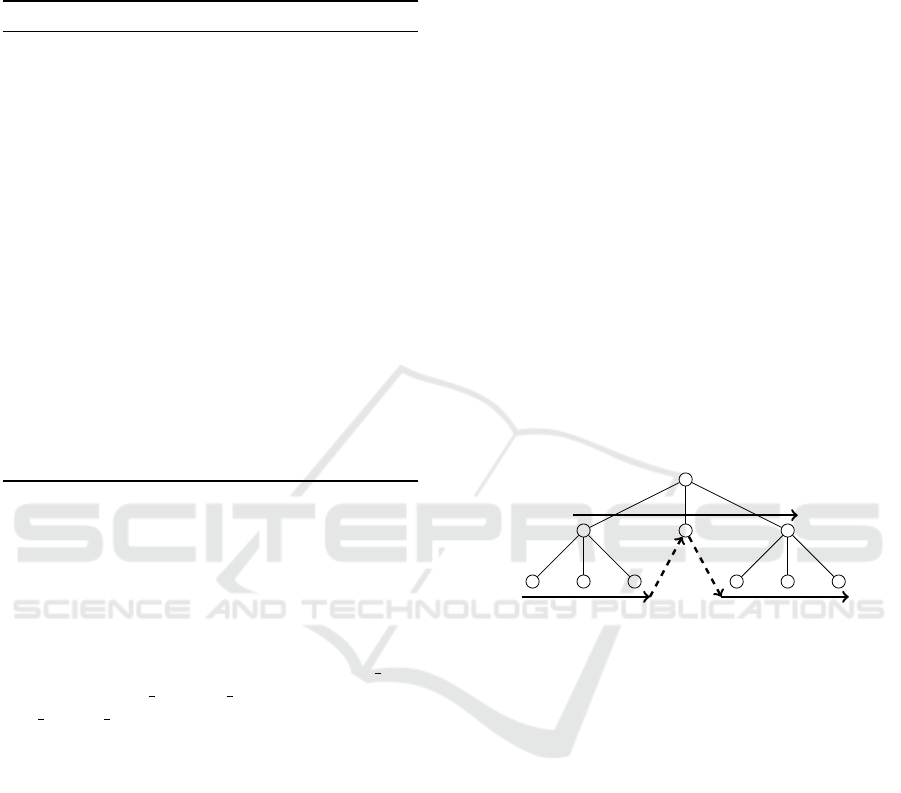
Table 1: Possible combinations of parameters. In the
SHAPE column: F = Forest; T = Tree; S = Separable; A =
Agreement; P = Path; In the GAP and MATCH columns: T
= True; F = False.
SHAPE GAP MATCH DESCRIPTION
F T F Ta
¨
ı (Ta
¨
ı, 1979)
F T T
F F F
F F T
T T F Identical to Ta
¨
ı distance.
T T T
T F F Identical to A-F-F.
T F T Identical to A-F-T.
S T F Constrained
(Zhang, 1995)
S T T
S F F
S F T
A T F Degree-two
(Zhang et al., 1996)
A T T
A F F Identical to T-F-F.
A F T Identical to T-F-T.
P T F
P T T
P F F
P F T
4.4 Combinations of Parameters
Table 1 shows the possible combinations of para-
meter values. For convenience of expression, we
represent each combination by the three capitals
of the parameter values selected. For example,
F-F-T represents the combination of SHAPE TYPE
= Forest, INTER VERTEX GAP = False and EX-
ACT LABEL MATCH = True.
Three of the distances in Table 1 are known
in the literature: F-T-F represents the Ta
¨
ı distance
(Ta
¨
ı, 1979); S-T-F represents the constrained distance
(Zhang, 1995); A-T-F represents the degree-two dis-
tance (Zhang et al., 1996). The remainder are novel
edit distances first introduced in this paper.
Also, some of them are identical to each other. To
be precise, since trees that do not allow inter-vertex
gaps are always agreement trees, T-F-F and T-F-T
are identical to A-F-F and A-F-F, respectively.
5 A COMPREHENSIVE
COMPARISON OF THE
MAPPING DISTANCE
MEASURES
5.1 Rooted Ordered Trees
To compute mapping distances efficiently, we further
assume that trees are rooted ordered trees.
When an total order is given to the children of
every parent vertex of a tree, the tree is called an roo-
ted ordered tree. The order is called a sibling order.
The sibling order can be easily extended to a left-right
order so that, given two vertices in a rooted ordered
tree, they are either in the ancestor-descendant rela-
tion or the left-right relation (Fig. 6).
When considering mapping distances between
rooted ordered trees, partial one-to=one mappings
(traces) that we consider must preserve not only the
ancestor-descendant order but also the left-right or-
der: x
1
is located left to x
2
in Dom(τ) ⊆ X, iff τ(x
1
) is
located left to τ(x
2
) in Y .
Figure 6: A rooted ordered tree: A sibling order (solid ar-
rows) and an extended left-right order (dashed arrows).
When trees are not ordered, in other words, when
they are rooted but unordered trees, it is known that
computing their edit distances is not necessarily trac-
table (Yamamoto et al., 2014).
On the other hand, when we assume that trees are
ordered, for all of the edit distances listed in Table 1,
there are efficient algorithms to compute them.
In the literature, the problem of computing
Ta
¨
ı edit distances has been known to have heavy
computational complexity, and much effort has been
made to improve efficiency. Zhang and Shasha
(Zhang and Shasha, 1989) proposed an algorithm of
O(|X||Y |min{w(X), h(X)}min{w(Y ),h(Y )})-time,
where |X |, w(X ) and h(X) denote the number of
vertices, the width (the number of leaves) and the
height (the length of the longest path from the
root to a leaf) of X. Klein (Klein, 1998) improved
the efficiency to O(|X|
2
|Y | log |Y |)-time by taking
advantage of decomposition strategies (Dulucq and
Touzet, 2003). Demaine et al. (Demaine et al., 2006)
further optimized this technique and presented an
algorithm of O(|X|
3
)-time. When we only look at
ICAART 2018 - 10th International Conference on Agents and Artificial Intelligence
270
the asymptotic evaluations, Demaine’s algorithm
looks the fastest, but it easily lapses into the worst
case. Therefore, the algorithm of Zhang and Shasha
in fact outperforms Demaine’s algorithm in many
practical cases. In this regard, RTED, an algorithm
that Pawlik and Augsten (Pawlik and Augsten, 2011)
have developed, not only has the same asymptotic
complexity as Demaine’s algorithm but also almost
always outperforms the competitors in practice.
For the constrained distance (Zhang, 1995) and
the degree-two distance (Zhang et al., 1996), effi-
cient algorithms to compute them in O(|X||Y |)-time
are presented in their original papers.
5.2 Algorithms
Fig. 7 to 11 give algorithms to compute the edit
distances listed in Table 1 except for those already
known.
The function c(x, y) for trees x and y is defined as
follows:
c(x, y) =
0, if `(rt(x)) = `(rt(y));
1, if `(rt(x)) 6= `(rt(y))
and ELM = False;
∞, if `(rt(x)) 6= `(rt(y))
and ELM = True.
`(rt(x)) denotes the label of the root of x and ELM
stands for EXACT LABEL MATCH.
In the diagrams of the figures, for a tree, the met-
hod .children takes the children of the root of the
tree and return as an array of trees. The order in the
array is identical to the sibling order.
The algorithm is expressed as pseudo-codes
using an imaginary programming language similar to
SCALA (https://scala-lang.org). For example, for an
array of trees the method .head returns the first tree
of the array, while the method .tail returns the new
array of trees after eliminating the first tree. Also,
the operator ++ indicates a simple concatenation of ar-
rays. The function ff* computes edit distances of the
types of F-F-F and F-F-T. The difference between
them as algorithms is only the value of c(x,y) used
when the labels `(rt(x)) and `(rt(y)) are different.
The asymptotic estimations of the time complex-
ity of these algorithms are O(|X|
2
|Y |
2
) for ff*, tt*
and tf* and O(|X||Y |) for the others. These complex-
ities might be improved taking advantages of the met-
hod used in (Pawlik and Augsten, 2011) and (Kimura
and Kashima, 2012). In (Kimura and Kashima, 2012),
a linear-time algorithm to compute subpath kernels is
presented. The algorithm leverages a list of all the
suffixes ordered in the lexicographical order: A suffix
ff*(x: Array[Tree], y: Array[Tree]): Int = {
if(x.isEmpty) return y.size
if(y.isEmpty) return x.size
t = x.head; u = y.head
v0 = c(t, u) + sub(t.children, u.children)
+ ff*(x.tail, y.tail)
v1 = ff*(t.children ++ x.tail, y) + 1
v2 = ff*(x, u.children ++ y.tail) + 1
return min(v0, v1, v2)
}
sub(x: Array[Tree], y: Array[Tree]): Int = {
if(x.isEmpty) return y.size
if(y.isEmpty) return x.size
t = x.head; u = y.head
v0 = c(t, u) + sub(t.children, u.children)
+ ff*(x.tail, y.tail)
v1 = e(x.tail, y) + t.size
v2 = e(x, y.tail) + u.size
return min(v0, v1, v2)
}
Figure 7: Algorithms for F-F-F and F-F-T.
tt*(x: Tree, y: Tree) => Int = {
v0 = c(x, y) + tt*(x.children, y.children)
v1 = x.children.map(t => sub(t, y) + x.size - t.size)
v2 = y.children.map(t => sub(x, t) + y.size - t.size)
v3 = x.size + y.size
return min(v0, min(v1), min(v2), v3)
}
sub(x: Array[Tree], y: Array[Tree]): Int = {
if(x.isEmpty) return y.size
if(y.isEmpty) return x.size
t = x.head; u = y.head
v0 = c(t, u) + sub(t.children, u.children)
+ sub(x.tail, y.tail)
v1 = sub(t.children ++ x.tail, y) + 1
v2 = sub(x, u.children ++ y.tail) + 1
return min(v0, v1, v2).min
}
Figure 8: Algorithms for T-T-F and T-T-T.
tf*(x: Tree, y: Tree) => Int = {
v0 = c(x, y) + sub (x.children, y.children)
v1 = x.children.map(t => tf*(t, y) + x.size - t.size)
++ Array(x.size + y.size)
v2 = y.children.map(t => tf*(x, t) + y.size - t.size)
++ Array(x.size + y.size)
return min(v0, min(v1), min(v2))
}
sub(x: Array[Tree], y: Array[Tree]): Int = {
if(x.isEmpty) return y.size
if(y.isEmpty) return x.size
t = x.head; u = y.head
v0 = c(t, u) + sub(t.children, u.children)
+ sub(x.tail, y.tail)
v1 = d(x.tail, y) + t.size
v2 = d(x, y.tail) + u.size
return min(v0, v1, v2)
}
Figure 9: Algorithms for T-F-F and T-F-T.
The Mapping Distance – a Generalization of the Edit Distance – and its Application to Trees
271

pt*(x: Tree, y: Tree) => Int = {
v0 = c(x, y) + x.size + y.size - 2 +
(Array(0) +: x.children.flatMap(t =>
y.children.map(u => pt*(t, u) - t.size - u.size)))
v1 = x.children.map(t => pttf(t, y) + x.size - t.size)
++ Array(x.size + y.size)
v2 = y.children.map(t => pttf(x, t) + y.size - t.size)
++ Array(x.size + y.size)
return min(min(v0), min(v1), min(v2))
}
Figure 10: Algorithms for P-T-F and P-T-T.
pf*: (x: Tree, y: Tree): Int = {
v0 = sub(x, y)
v1 = x.children.map(t => pf*(t, y) + x.size - t.size)
v2 = y.children.map(t => pf*(x, t) + y.size - t.size)
v3 = x.size + y.size
return min(v0, min(v1), min(v2), v3)
}
sub(x: Tree, y: Tree): Int = {
return c(x, y) + x.size + y.size - 2 +
min((Array(0) ++ x.children.flatMap(t =>
y.children.map(u => sub(t, u) - t.size - u.size))))
Figure 11: Algorithms for P-F-F and P-F-T.
is a string of labels of a contiguous path from a vertex
to the root of the tree.
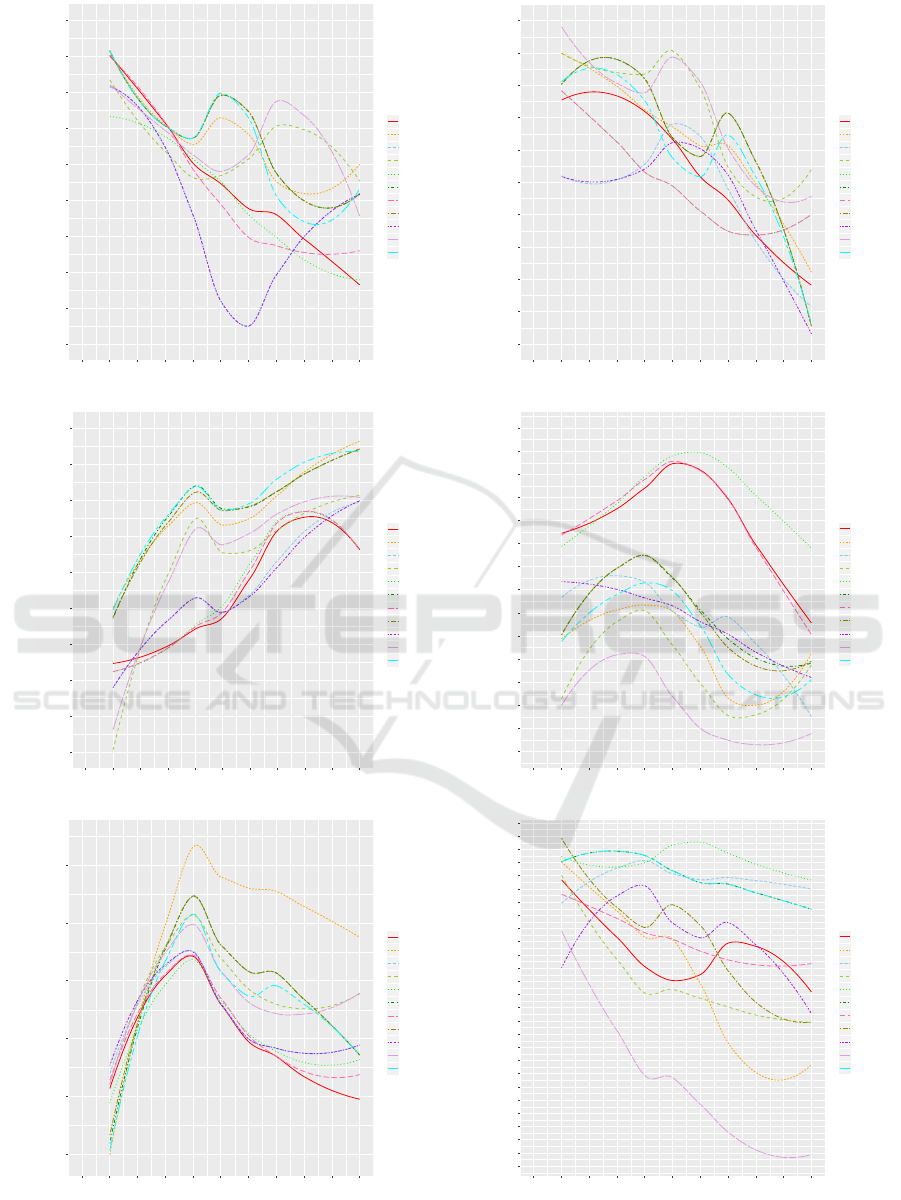
5.3 Comparison Results
In the following, we see the results of experiments
using six datasets. We ran five-fold cross validation
with the k-NN algorithm changing k from 1 to 10, and
then, measured accuracy scores (
TP+TN
TP+FP+FN+TN
). The
edit distance measures whose SHAPE TYPE parameter
is PATH did not show good results for all the datasets
tested, we exclude them from the explanation.
5.3.1 Colon-Cancer Dataset
The COLON-CANCER dataset was retrieved from the
KEGG/GLYCAN database (Hashimoto et al., 2006),
and specifies 134 glycan trees annotated relating to
the disease of colon cancer. As Fig. 12 (a) shows,
although the T-T-T, A-T-T, A-T-F (degree-two) and
S-T-F (constrained) distances show the highest accu-
racy, the novel two outperform the known two on
average across all k.
5.3.2 Cystic-Fibrosis Dataset
This dataset was also retrieved from the
KEGG/GLYCAN database. It contains 160 gly-
can trees annotated relating to the disease of
cystic-fibrosis. As Fig. 12 (b) shows, the T-F-T
distance shows the highest accuracy, which is novel
introduced in this paper.
5.3.3 Leukemia Dataset
This dataset was also retrieved from the
KEGG/GLYCAN database. It contains 422 trees
annotated relating to the disease of leukemia. As
Fig. 12 (c) shows, the A-T-T, T-T-T and L-T-T
distances show the highest accuracy. All of them
require exact label match, and therefore, are novel.
5.3.4 Syntactic Dataset
This dataset is the dataset PropBank provided
in (Moschitti, ). It contains 225 parse trees labeled
with two syntactic role classes for modeling the syn-
tactic/semantic relation between a predicate and the
semantic roles of its arguments in a sentence. As
Fig. 12 (d) shows, the F-T-F (Ta
¨
ı) distance shows
the highest accuracy, and the S-T-F (constrained) and
A-T-F (degree-two) distances follow. All of them are
known in the literature.
5.3.5 Web Access Dataset
This dataset was the one used in (Zaki and Aggarwal,
2006), and consists of 810 trees representing web-
page accesses by users, and the annotation is based
on whether the user is from a .edu site or not. As
Fig. 12 (e) shows, the A-T-T distance outperforms the
others in terms of both the highest accuracy and the
average. The A-T-T distance has been introduced in
this paper.
5.3.6 Phishing Dataset
We generated this dataset for this experiment. We
collected 73 URL of phishing sites from PhishTank,
(https://www.phishtank.com/), and 65 URL of au-
thentic sites independently. From the collected URL,
we generated DOM trees to form this dataset. As
Fig. 12 (f) shows, the F-T-F (Ta
¨
ı) distance shows the
highest accuracy, and the F-F-F and T-T-T distances
follow.
5.4 Summary
The table below shows the averaged ranks with re-
spect to the highest accuracy scores across the six da-
tasets.
We should remark that the distances of the *-T-T
type monopolize the top four. Hence, distances with
traces that allow gaps between vertices and require
exact match between labels can be more accurate. Of
ICAART 2018 - 10th International Conference on Agents and Artificial Intelligence
272
A A
A A
A A
A A
A A
B B
B B
B B
B B
B B
C C
C C
C C
C C
C C
D D
D D D D
D D
D D
E E
E E
E E
E E
E E
F F
F F
F F
F F F F
K K
K K
K K
K K K K
L L
L L
L L
L L L L
M M
M M
M M
M M
M M
N N
N N
N N
N N
N N
P P
P P
P P
P P
P P
0.84
0.85
0.86
0.87
0.88
0.89
0.90
0.91
0.92
0.93
0 1 2 3 4 5 6 7 8 9 10
k
accuracy
metric
A
B
C
D
E
F
K
L
M
N
P
atf
att
fff
fft
ftf
ftt
stf
stt
tff
tft
ttt
(a) COLON-CANCER
A A A A
A A
A A
A A
B B
B B
B B
B B
B B
C C C C
C C
C C
C C
D D
D D
D D
D D
D D
E E
E E
E E
E E
E E
F F
F F
F F
F F
F F
K K
K K
K K
K K
K K
L L
L L
L L
L L
L L
M M M M
M M
M M
M M
N N
N N
N N
N N
N N
P P P P
P P
P P
P P
0.63
0.64
0.65
0.66
0.67
0.68
0.69
0.70
0.71
0.72
0.73
0 1 2 3 4 5 6 7 8 9 10
k
accuracy
metric
A
B
C
D
E
F
K
L
M
N
P
atf
att
fff
fft
ftf
ftt
stf
stt
tff
tft
ttt
(b) CYSTIC-FIBROSIS
A A
A A
A A
A A
A A
B B
B B
B B
B B
B B
C C
C C
C C
C C
C C
D D
D D
D D
D D
D D
E E
E E
E E
E E
E E
F F
F F
F F
F F
F F
K K
K K
K K
K K
K K
L L
L L
L L
L L
L L
M M
M M
M M
M M
M M
N N
N N N N
N N
N N
P P
P P
P P
P P
P P
0.785
0.795
0.805
0.815
0.825
0.835
0.845
0.855
0.865
0.875
0 1 2 3 4 5 6 7 8 9 10
k
accuracy
metric
A
B
C
D
E
F
K
L
M
N
P
atf
att
fff
fft
ftf
ftt
stf
stt
tff
tft
ttt
(c) Leukemia
A A
A A
A A
A A
A A
B B
B B
B B
B B
B B
C C
C C
C C C C
C C
D D
D D
D D
D D
D D
E E
E E
E E
E E
E E
F F
F F
F F
F F
F F
K K
K K
K K
K K
K KL L
L L
L L
L L L L
M M
M M
M M
M M
M M
N N
N N
N N
N N
N N
P P
P P
P P
P P
P P
0.70
0.71
0.72
0.73
0.74
0.75
0.76
0.77
0.78
0.79
0.80
0.81
0.82
0.83
0.84
0 1 2 3 4 5 6 7 8 9 10
k
accuracy
metric
A
B
C
D
E
F
K
L
M
N
P
atf
att
fff
fft
ftf
ftt
stf
stt
tff
tft
ttt
(d) Syntactic
A A
A A
A A
A A
A A
B B
B B
B B
B B
B B
C C
C C
C C
C C
C C
D D
D D
D D
D D
D D
E E
E E
E E
E E E E
F F
F F
F F
F F
F F
K K
K K
K K
K K
K K
L L
L L
L L
L L
L LM M
M M
M M
M M
M M
N N
N N
N N
N N
N N
P P
P P
P P P P
P P
0.80
0.81
0.82
0.83
0.84
0.85
0 1 2 3 4 5 6 7 8 9 10
k
accuracy
metric
A
B
C
D
E
F
K
L
M
N
P
atf
att
fff
fft
ftf
ftt
stf
stt
tff
tft
ttt
(e) Web-Access
A A
A A
A A
A A
A A
B B
B B
B B
B B B B
C C
C C
C C C C
C CD D
D D
D D
D D
D D
E E
E E
E E
E E
E E
F F
F F
F F
F F
F F
K K
K K
K K
K K K K
L L
L L
L L
L L
L L
M M
M M
M M
M M
M M
N N
N N
N N
N N
N N
P P
P P
P P
P P
P P
0.55
0.56
0.57
0.58
0.59
0.60
0.61
0.62
0.63
0.64
0.65
0.66
0.67
0.68
0.69
0.70
0.71
0.72
0.73
0.74
0.75
0.76
0.77
0.78
0.79
0.80
0.81
0 1 2 3 4 5 6 7 8 9 10
k
accuracy
metric
A
B
C
D
E
F
K
L
M
N
P
atf
att
fff
fft
ftf
ftt
stf
stt
tff
tft
ttt
(f) Phishing
Figure 12: Comparison in accuracy.
The Mapping Distance – a Generalization of the Edit Distance – and its Application to Trees
273

FTT STT ATT TTT TFT ATF
3.2 3.2 3.6 4.6 6.9 6.9
FFT STF FTF FFF TFF
6.9 7.2 7.4 7.7 8.4
course, all of them are novel distance measures intro-
duced in this paper. Furthermore, the following shows
the p-values when we perform the Hommel test let-
ting F-T-T be the control.
FTT STT ATT TTT TFT ATF
– 1.00 0.81 0.84 0.16 0.16
FFT STF FTF FFF TFF
0.14 0.10 0.10 0.07 0.04
We see that there is a clear line between the *-T-T
type and the others: with the significance level of
10%, the superiority of the F-T-T (and S-T-T) dis-
tance to the S-T-F (constrained), F-T-F (Ta
¨
ı), F-F-F
and T-F-F distances is proven statistically significant;
For the A-T-F (degree-two) and T-F-T distances, alt-
hough we cannot reject the null hypothesis, the p-
values are as small as 16%, much smaller than 84%
for the T-T-T distance.
6 CONCLUSION
We have shown that viewing edit distance measures
from a view point of properties of their associated tra-
ces is useful. In particular, by using particular proper-
ties of traces as parameters to describe edit distance
measures, we not only can deal with edit distances
measures consistently but also can engineer new me-
asures systematically. In fact, taking rooted trees as an
example, we have introduced three independent para-
meters, and have shown that the parameters determine
16 edit distance measures. Surprisingly, only three
among them had been known in the literature, and
all the remainder were novel. Furthermore, through
experiments to measure predictive accuracy of each
combination of one of the 16 measures and the k-
NN classifier, we have discovered that a certain novel
class of edit distance measures can perform the best.
The measures belonging to the class are significantly
different from the edit distance measures known in
the literature, since the cost to replace a label with a
different label is set as infinity. This mandates the as-
sociated traces to preserve labels of vertices.
7 ACKNOWLEDGMENTS
This work was partially supported by the Grant-in-
Aid for Scientific Research (JSPS KAKENHI Grant
Number 16K12491 and 17H00762) from the Japan
Society for the Promotion of Science.
REFERENCES
Collins, M. and Duffy, N. (2001). Convolution kernels for
natural language. In Advances in Neural Information
Processing Systems 14 [Neural Information Proces-
sing Systems: Natural and Synthetic, NIPS 2001], pa-
ges 625–632. MIT Press.
Demaine, E. D., Mozes, S., Rossman, B., and Weimann, O.
(2006). An optimal decomposition algorithm for tree
edit distance. ACM Trans. Algo., 6.
Dulucq, S. and Touzet, H. (2003). Analysis of tree edit
distance algorithms. In the 14th annual symposium on
Combinatorial Pattern Matching (CPM), pages 83 –
95.
Hashimoto, K., Goto, S., Kawano, S., Aoki-Kinoshita,
K. F., and Ueda, N. (2006). KEGG as a glycome in-
formatics resource. Glycobiology, 16:63R – 70R.
Kao, M.-Y., Lam, T.-W., Sung, W.-K., and Ting, H.-F.
(2007). An even faster and more unifying algorithm
for comparing trees via unbalanced bipartite matc-
hings.
Kimura, D. and Kashima, H. (2012). Fast computation of
subpath kernel for trees. In ICML.
Klein, P. N. (1998). Computing the edit-distance between
unrooted ordered trees. LNCS, 1461:91–102. ESA’98.
Kuboyama, T., Shin, K., Miyahara, T., and Yasuda, H.
(2005). A theoretical analysis of alignment and edit
problems for trees. In Proc. of Theoretical Computer
Science, The 9th Italian Conference, Lecture Notes in
Computer Science 3701, pages 323–337.
Levenshtein, V. I. (1966). Binary codes capable of cor-
recting deletions, insertions, and reversals. Soviet
Physics Doklady, 10(8):707 – 710.
Lu, C. L., Su, Z. Y., and Tang, G. Y. (2001). A New Measure
of Edit Distance between Labeled Trees. In LNCS, vo-
lume 2108, pages pp. 338–348. Springer-Verlag Hei-
delberg.
Moschitti, A. Example data for TREE KERNELS
IN SVM-LIGHT. http://disi.unitn.it/moschitti/Tree-
Kernel.htm.
Neuhaus, M. and Bunke, H. (2007). Bridging the gap bet-
ween graph edit distance and kernel machines. World
Scientific.
Pawlik, M. and Augsten, N. (2011). Rted: A robust algo-
rithm for the tree edit distance. In Proceedings of the
VLDB Endowment, volume 5, pages 334–345.
Shin, K. (2015). Tree edit distance and maximum
agreement subtree. Inf. Process. Lett., 115(1):69–73.
Ta
¨
ı, K. C. (1979). The tree-to-tree correction problem. jour-
nal of the ACM, 26(3):422–433.
ICAART 2018 - 10th International Conference on Agents and Artificial Intelligence
274

Wang, J. T. L. and Zhang, K. (2001). Finding similar con-
sensus between trees: an algorithm and a distance
hierarchy. Pattern Recognition, 34:127–137.
Yamamoto, Y., Hirata, K., and Kuboyama, T. (2014). Trac-
table and intractable variations of unordered tree edit
distance. Int. J. Found. Comput. Sci, 25(3):307–330.
Zaki, M. J. and Aggarwal, C. C. (2006). XRules: An ef-
fective algorithm for structural classification of XML
data. Machine Learning, 62:137–170.
Zhang, K. (1995). Algorithms for the constrained edi-
ting distance between ordered labeled trees and related
problems. Pattern Recognition, 28(3):463–474.
Zhang, K. and Shasha, D. (1989). Simple fast algorithms
for the editing distance between trees and related pro-
blems. SIAM journal of Computing, 18(6):1245 –
1262.
Zhang, K., Wang, J. T. L., and Shasha, D. (1996). On the
editing distance between undirected acyclic graphs.
International Journal of Foundations of Computer
Science, 7(1):43–58.
The Mapping Distance – a Generalization of the Edit Distance – and its Application to Trees
275
