
On the Taut String Interpretation of the One-dimensional
Rudin–Osher–Fatemi Model
Niels Chr Overgaard
Centre for Mathematical Sciences, Lund University, S
¨
olvegatan 18A, 221 00 Lund, Sweden
Keywords:
Total Variation Minimization, Taut String, Denoising, Regression Splines, Lewy–Stampacchia Inequality,
Sub-modularity, Moreau-Yosida Approximation, Isotonic Regression.
Abstract:
A new proof of the equivalence of the Taut String Algorithm and the one-dimensional Rudin–Osher–Fatemi
model is presented. Based on duality and the projection theorem in Hilbert space, the proof is strictly ele-
mentary. Existence and uniqueness of solutions (in the continuous case) to both denoising models follow as
by-products. The standard convergence properties of the denoised signal, as the regularizing parameter tends
to zero, are recalled and efficient proofs provided. Moreover, a new and fundamental estimate on the denoised
signal is derived. It implies, among other things, the strong convergence (in the space of functions of bounded
variation) of the denoised signal to the in-signal as the regularization parameter vanishes.
1 INTRODUCTION
In 2017 it was 25 years ago Leonid Rudin, Stanley
Osher and Emad Fatemi proposed their now classical
model for edge-preserving denoising of images (Ru-
din et al., 1992). The present paper will investi-
gate the properties of the one-dimensional version of
the Rudin-Osher-Fatemi (ROF) model: To a given
(noisy) signal f ∈ L
2
(I), defined on a bounded inter-
val I = (a, b), associate the (ROF) functional
E
λ
(u) = λ
Z
b
a
|u
0
(x)|dx +
1
2
Z
b
a
( f (x) − u(x))
2
dx ,
where λ > 0 is a parameter. Define the denoised sig-
nal as the function u
λ
∈ BV (I) which minimizes this
energy, i.e.,
u
λ
:= arg min
u∈BV (I)
E
λ
(u) . (1)
The first term in the ROF-functional is λ times the
total variation
R
b
a
|u
0
|dx of the function u and BV (I)
denotes the set of functions on I with finite total varia-
tion. Precise definitions will be given below, in Secti-
ons 2 and 3.
The one-dimensional ROF model is compared to
the Taut string algorithm—an alternative method for
denoising of signals with applications in statistics,
non-parametric estimation, real-time communication
systems and stochastic analysis. In the continuous
setting, for analogue signals, the Taut string algorithm
can be stated in the following manner (cf. Figure 1):
Algorithm 1: The Taut String Algorithm.
INPUT: A bounded interval I = (a,b), a (noisy) signal
f ∈ L
2
(I) and a parameter λ > 0.
OUTPUT: The denoised signal f
λ
∈ L
2
(I).
STEP 1. Compute the cumulative signal,
F(x) =
Z
x
a
f (t)dt , x ∈
I = [a, b].
STEP 2. Set
T
λ
=
n
W ∈ H
1
(I) : W (a) = F(a), W (b) = F(b),
and F − λ ≤ W ≤ F +λ
o
.
(The set of L
2
-functions with weak derivatives in L
2
and graphs lying within a tube around F of width λ.)
STEP 3. Compute the unique minimizer W
λ
∈ T
λ
(the
‘Taut string’) of the energy
min
W ∈T
λ
E(W ) :=
1
2
Z
b
a
W
0
(x)
2
dx . (2)
STEP 4. Set f
λ
= W
0
λ
(distributional derivative.)
END.
The taut string algorithm has been extensively stu-
died in the discrete setting by (Mammen and van de
Geer, 1997; Davies and Kovac, 2001) and (D
¨
umbgen
and Kovac, 2009). Very recently, using methods from
Overgaard, N.
On the Taut String Interpretation of the One-dimensional Rudin–Osher–Fatemi Model.
DOI: 10.5220/0006720402330244
In Proceedings of the 7th International Conference on Pattern Recognition Applications and Methods (ICPRAM 2018), pages 233-244
ISBN: 978-989-758-276-9
Copyright © 2018 by SCITEPRESS – Science and Technology Publications, Lda. All rights reserved
233

interpolation theory (Peetre’s K-functional and the
notion of invariant K-minimal sets), Setterqvist has
investigated the limits to which taut string methods
may be extended (Setterqvist, 2016).
In its original formulation, the Taut string algo-
rithm instruct us to find the solution of the shortest
path problem
min
W ∈T
λ
L(W ) :=
Z
b
a
q
1 +W
0
(x)
2
dx , (3)
hence the epithet ‘taut string’. However, the ‘stret-
ched rubber band’-energy E in step 3 of the algorithm
is not only easier to handle analytically, it also has
precisely the same solution as (3). While this is intui-
tively clear from our everyday experience with rub-
ber bands and strings, the assertion is, mathematically
speaking, not equally self-evident so a proof is offered
in Appendix A.
The main purpose of this paper, the first of two,
is to present a new, elementary proof of the following
remarkable result:
Theorem 1. The Taut string algorithm and the ROF
model yield the same solution; f
λ
= u
λ
.
This is not new; a discrete version of this theorem
was proved in (Mammen and van de Geer, 1997) and
in (Davies and Kovac, 2001). In the continuum set-
ting, the equivalence result was explicitly stated and
proved in (Grassmair, 2007). There is also an exten-
sive treatment in (Scherzer et al., 2009, Ch. 4). In-
deed, a few years earlier (Hinterm
¨
uller and Kunisch,
2004, p.7), in a brief (but inconclusive) remark, refer
to the close relation between the ROF model and the
Taut string algorithm.
The second main result of the paper, whose proof
we give in Section 6, is the following “fundamental”
estimate on the denoised signal:
Theorem 2. If the signal f belongs to BV (I) then, for
any λ > 0, the denoised signal u
λ
satisfies the inequa-
lity
−( f
0
)
−
≤ u
0
λ
≤ ( f
0
)
+
, (4)
where ( f
0
)
+
and ( f
0
)
−
denote the positive and the
negative variations, respectively, of f
0
(distributional
derivative).
Just like f
0
, the derivative u
0
λ
is computed in the
distributional sense and is, in general, a signed mea-
sure. Recall that ( f
0
)
+
and ( f
0
)
−
are finite positive
measures satisfying f
0
= ( f
0
)
+
− ( f
0
)
−
, see e.g. (Ru-
din, 1986, Sec. 6.6). As an example, compute the
derivatives of f and u
λ
= f
λ
as shown in Figure 1.
The proof of the theorem is based on (an extension of)
the Lewi–Stampacchia-inequality (Lewy and Stam-
pacchia, 1970) and uses the Taut String-interpretation
of the ROF model (Theorem 1) in an essential way.
A significant consequence of Theorem 2 is that
for an in-signal f belonging to BV (I) we get u
λ
→ f
strongly in BV (I) as λ → 0+ . The usual Moreau–
Yosida approximation result, see e.g. (Ambrosio
et al., 2000, Ch. 17), only gives the weaker u
λ
→ f in
L
2
(I) and
R
I
|u
0
λ
|dx →
R
I
| f
0
|dx as λ tends to zero.
Further contributions of the paper are: i) The re-
derivation some known properties of the ROF model
(Propositions 2) and ii) proof of some precise results
on the rate of convergence of u
λ
→ f as λ tends to
zero Propositions 3 and 4—collecting all such result
in one place! iii) A new and slick proof of the (known)
fact that u
λ
is a semi-group with respect to λ (Propo-
sition 8). iv) Finally we indicated how our method of
proof can be modified and applied to the problem of
isotonic regression.
The paper is based on the author’s preprint (Over-
gaard, 2017) and is completely theoretical. All exam-
ples, including the ones in the figures, are computed
by hand using the taut string interpretation. Howe-
ver, we predict that the theory developed can be used
to construct new fast non-iterative algorithms for de-
noising using the ROF-model or, at least, can be used
to shed new light on existing such algorithms such
as (Condat, 2013).
2 OUR ANALYSIS TOOLBOX
Throughout this paper I denotes an open, bounded
interval (a, b), where a < b are real numbers, and
¯
I = [a, b] is the corresponding closed interval.
C
1
0
(I) denotes the space of continuously differen-
tiable (test-)functions ξ : I → R with compact support
in I, and C(
¯
I) is the space of continuous functions on
the closure of I.
For 1 ≤ p ≤ ∞, L
p
(I) denotes the Lebesgue space
of measurable functions f : I → R with finite p-norm;
k f k
p
:=
R
b
a
| f (x)|
p
dx
1/p
< ∞, when p is finite,
and k f k
∞
= esssup
x∈I
| f (x)| < ∞ when p = ∞. The
space L
2
(I) is a Hilbert space with the inner product
h f , gi = h f ,gi
L
2
(I)
:=
R
b
a
f (x)g(x) dx and the corre-
sponding norm k f k :=
q
h f , f i
L
2
(I)
= k f k
2
.
We are going to need the Sobolev spaces over L
2
:
H
1
(I) =
u ∈ L
2
(I) : u
0
∈ L
2
(I)
,
were u
0
denotes the distributional derivative of u.
This is a Hilbert space with inner product hu, vi
H
1
:=
hu,vi + hu
0
,v
0
i and norm kuk
H
1
= (ku
0
k
2
2
+ kuk
2
2
)
1/2
.
Any u ∈ H
1
(I) can, after correction on a set of mea-
sure zero, be identified with a unique function in C(
¯
I).
In particular, a unique value u(x) can be assigned to u
for every x ∈
¯
I.
ICPRAM 2018 - 7th International Conference on Pattern Recognition Applications and Methods
234

x
y
1
−1
f
a
b
(a) The input signal f .
x
y
λ
−λ
F
F +λ
F −λ
b
(b) The cumulative signal F and the tube T
λ
.
x
y
λ
−λ
b
W
λ
(c) The taut string W
λ
.
x
y
1
−1
f = F
0
f
λ
= W
0
λ
a
b
(d) The denoised signal f
λ
together with the input sig-
nal.
Figure 1: A graphical illustrations of the steps in the Taut string algorithm applied to a piecewise constant signal.
The following subspace of H
1
(I) plays an impor-
tant role in our analysis:
H
1
0
(I) =
u ∈ H
1
(I) : u(a) = 0 and u(b) = 0
.
Here hu,vi
H
1
0
(I)
:=
R
b
a
u
0
(x)v
0
(x)dx defines an inner
product on H
1
0
(I) whose induced norm kuk
H
1
0
(I)
=
ku
0
k
2
is equivalent to the norm inherited from H
1
(I).
Finally, let H be a (general) real Hilbert space with
inner product between u, v ∈ H denoted by hu,vi and
the corresponding norm kuk =
p
hu,ui. The follo-
wing result is standard (Br
´
ezis, 1999, Th
´
eor
`
eme V.2):
Proposition 1 (Projection Theorem). Let K ⊂ H be
a non-empty closed convex set. Then for every ϕ ∈ H
there exists a unique point u ∈ K such that
kϕ − uk = min
v∈K
kϕ − vk.
Moreover, the minimizer u is characterized by the fol-
lowing property:
u ∈ K and hϕ − u,v − ui ≤ 0, for all v ∈ K.
The point u is called the projection of ϕ onto K, and
is denoted u = P
K
(ϕ).
3 PRECISE DEFINITION OF THE
ROF MODEL
The expression
R
I
|u
0
|dx for the total variation, makes
sense for u ∈ H
1
(I) but is otherwise merely a conve-
nient symbol. A more general and precise definition
is needed; one which works when u
0
does not exist
in the classical sense. The standard way to define the
total variation is via duality: For u ∈ L
1
(I) set
J(u) = sup
n
Z
b
a
u(x)ξ
0
(x)dx :
ξ ∈ C
1
0
(I), kξk
∞
≤ 1
o
. (5)
If J(u) < ∞, u is said to be a function of bounded
variation on I, and J(u) is called the total variation
of u (using the same notation as (Chambolle, 2004)).
The set of all integrable functions on I of bounded
variation is denoted BV (I), that is, BV (I) =
u ∈
L
1
(I) : J(u) < ∞
. This becomes a Banach space
when equipped with the norm kuk
BV
:= J(u)+kuk
L
1
.
Notice that, as already mentioned, if u ∈ H
1
(I) then
J(u) =
R
I
|u
0
|dx < ∞, so u ∈ BV (I).
Let us illustrate how the definition works for a
function with a jump discontinuity:
On the Taut String Interpretation of the One-dimensional Rudin–Osher–Fatemi Model
235

Example 1. Let u(x) = sign(x) on the interval I =
(−1,1). For any ξ ∈ C
1
0
(I), satisfying |ξ(x)| ≤ 1 for
all x ∈ I, we have
Z
1
−1
u(x)ξ
0
(x)dx
=
Z
1
0
ξ
0
(x)dx −
Z
0
−1
ξ
0
(x)dx = −2ξ(0) ≤ 2,
where equality holds for any admissible ξ which
satisfies ξ(0) = −1. So J(u) = 2 and u ∈ BV (I), as
predicted by intuition.
In this example the supremum is attained by many
choices of ξ. This is not always the case; if u(x) = x
on I = (0, 1) then J(u) = 1, but the supremum is not
attained by any admissible test function.
The following lemma shows that the definition of
the total variation J and the space BV (I) can be moved
to a Hilbert space-setting involving L
2
and H
1
0
.
Lemma 3. Every u ∈ BV (I) belongs to L
2
(I) and
J(u) = sup
ξ∈K
hu,ξ
0
i
L
2
(I)
, (6)
where K = {ξ ∈ H
1
0
(I) : kξk
∞
≤ 1 }, which is a closed
and convex set in H
1
0
(I).
Proof. If u ∈ BV (I) then Sobolev’s lemma for functi-
ons of bounded variation, see (Ambrosio et al., 2000,
p. 152), ensures that u ∈ L
∞
(I). This in turn implies
u ∈ L
2
(I) because I is bounded. The (ordinary) So-
bolev’s lemma asserts that H
1
0
(I) is continuously em-
bedded in L
∞
(I). Since K is the inverse image under
the embedding map of the unit ball in L
∞
(I), which is
both closed and convex, we draw the conclusion that
K is closed and convex in H
1
0
.
It only remains to prove (6). Clearly J(u) cannot
exceed the right hand side because the set {ξ ∈ C
1
0
(I) :
kξk
∞
≤ 1 } is contained in K. To verify that equality
holds it is enough to prove the inequality
hu,ξ
0
i
L
2
(I)
≤ J(u)kξk
∞
, for all ξ ∈ H
1
0
(I), (7)
as it implies that the right hand side of (6) cannot ex-
ceed J(u). To do this, we first notice that the ine-
quality in holds for all ζ ∈ C
1
0
(I). This follows by
applying homogeneity to the definition of J(u). Se-
condly, if ξ ∈ H
1
0
(I) we can use that C
1
0
(I) is dense in
H
1
0
(I) and find functions ζ
n
∈ C
1
0
(I) such that ζ
n
→ ξ
in H
1
0
(I) (and in L
∞
(I) by the continuous embedding).
It follows that
hu,ξ
0
i
L
2
(I)
= lim
n→∞
hu,ζ
0
n
i
L
2
(I)
≤ J(u) lim
n→∞
kζ
n
k
∞
= J(u)kξk
∞
,
which establishes (7) and the proof is complete.
The inequality (7) combined with the Riesz repre-
sentation theorem (cf. e.g. (Ambrosio et al., 2000,
Thm. 1.54)) implies that the distributional derivative
u
0
of u ∈ BV (I) is a signed (Radon) measure µ on I,
and that we may write hu,ξ
0
i
L
2
(I)
=
R
I
ξdµ. This will
be useful later on.
We can now give the precise definition of the ROF
model: For any f ∈ L
2
(I) and any real number λ > 0
the ROF functional is the function E
λ
: BV (I) → R
given by
E
λ
(u) = λJ(u) +
1
2
k f − uk
2
L
2
(I)
. (8)
Denoising according to the ROF model is the map
L
2
(I) 3 f 7→ u
λ
∈ BV (I) defined by (1). To empha-
sise the role of the in-signal f we sometimes write
E
λ
( f ;u) instead of E
λ
(u). Well-posedness of the ROF
model is demonstrated in the next section.
4 EXISTENCE THEORY FOR
THE ROF MODEL
We begin with a simple observation: if u ∈ BV (I)
then J(u + c) = J(u) for any real constant c. This
property of the total variation has two important con-
sequences. First of all, E
λ
( f ;u) = E
λ
( f − c; u − c)
for any constant c. Taking c to be the mean value
of f shows that we may assume, as we do throug-
hout this paper, that the in-signal satisfies
R
I
f dx = 0.
This assumption implies that the cumulative signal
F(x) satisfies F(a) = F(b) = 0, hence F ∈ H
1
0
(I).
This plays an important role in our analysis. Se-
condly, since f has mean value zero, it is enough to
minimize E
λ
over the subspace of BV (I) consisting
of functions with mean value zero. To see this, let
P be the orthogonal projection (in L
2
(I)) onto this
subspace. An easy computation yields the identity
E
λ
(Pu) = E
λ
(u) −
1
2
ku − Puk
2
, which shows that u
can be a minimizer of E
λ
only if it belongs to the
range of P.
The following theorem contains the key result of
our paper.
Theorem 4. We have the equality
min
u∈BV (I)
E
λ
(u) = max
ξ∈K
1
2
n
k f k
2
L
2
(I)
− k f − λξ
0
k
2
L
2
(I)
o
,
(9)
with the minimum achieved by a unique u
λ
∈ BV (I)
and the maximum by a unique ξ
λ
∈ K. The two functi-
ons are related by the identity
u
λ
= f − λξ
0
λ
, (10a)
and satisfy
J(u
λ
) = hu
λ
,ξ
0
λ
i
L
2
(I)
. (10b)
ICPRAM 2018 - 7th International Conference on Pattern Recognition Applications and Methods
236

Moreover, if u
λ
6= 0, then kξ
λ
k
∞
= 1. Conversely, the
conditions (10a) and (10b) characterizes the solution;
if a pair of functions ¯u ∈ BV (I) and
¯
ξ ∈ K satisfy ¯u =
f −λ
¯
ξ
0
and J( ¯u) = h ¯u,
¯
ξ
0
i
L
2
(I)
, then ¯u = u
λ
and
¯
ξ = ξ
λ
.
This result is a special instance of the Fenchel–
Rockafellar theorem, see e.g. (Br
´
ezis, 1999, p. 11). It
is tailored with our specific needs in mind and will be
proved with our bare hands using the projection theo-
rem. The general version is used in (Hinterm
¨
uller and
Kunisch, 2004) in their analysis of the multidimensi-
onal ROF model (with the ‘Manhattan metric’). The
equality (9) has played an important role in the de-
velopment of numerical algorithms for total variation
minimization, both directly, as for instance in (Zhu
et al., 2007) or, indirectly, as in (Chambolle, 2004).
Before the proof starts, let us remind the reader of
the following general fact: If M and N are arbitrary
non-empty sets and Φ : M × N → R is any real valued
function, then it is easy to check that
inf
x∈M
sup
y∈N
Φ(x,y) ≥ sup
y∈N
inf
x∈M
Φ(x,y) , (11)
is always true. The use of inf’s and sup’s are impor-
tant, as neither the greatest lower bounds nor the least
upper bounds are necessarily attained.
Proof. Since E
λ
(u) = sup
ξ∈K
λhu,ξ
0
i +
1
2
k f − uk
2
it
follows from (11) that
inf
u∈BV (I)
E
λ
(u) ≥ sup
ξ∈K
n
inf
u∈BV (I)
λhu,ξ
0
i +
1
2
ku − f k
2
o
.
We first solve, for ξ ∈ K fixed, the minimization pro-
blem on the right hand-side. Expanding k f − uk
2
and
completing squares with respect to u yields:
λhu,ξ
0
i +
1
2
ku − f k
2
=
1
2
n
ku − ( f − λξ
0
)k
2
− k f − λξ
0
k
2
+ k f k
2
o
The right hand-side is clearly minimized by the L
2
(I)-
function u = f − λξ
0
and
inf
u∈BV (I)
E
λ
(u) ≥ sup
ξ∈K
1
2
n
k f k
2
− k f − λξ
0
k
2
o
(12)
holds. The maximization problem on the right hand
side is equivalent to
inf
ξ∈K
k f − λξ
0
k = inf
ξ∈K
kF
0
− λξ
0
k
= λ inf
ξ∈K
kλ
−1
F − ξk
H
1
0
(I)
. (13)
By Proposition 1, this problem has the unique solution
ξ
λ
= P
K
(λ
−1
F) ∈ K, so the supremum is attained in
(12). Now, let the function u
λ
be defined by (10a) in
the theorem. A priori, u
λ
belongs to L
2
(I), but we are
going to show that u
λ
∈ BV (I): The characterization
of ξ
λ
according in the projection theorem states that
ξ
λ
∈ K and h f − λξ
0
λ
,λξ
0
− λξ
0
λ
i ≤ 0 for all ξ ∈ K. If
we use the definition of u
λ
and divide by λ > 0 this
characterization becomes
hu
λ
,ξ
0
i ≤ hu
λ
,ξ
0
λ
i for all ξ ∈ K,
where the right hand-side is finite. It follows from the
definition of the total variation that u
λ
∈ BV (I) with
J(u
λ
) = hu
λ
,ξ
0
λ
i, as asserted in the theorem. (This
reasoning can be reversed; if (10b) is true then ξ
λ
is
the minimizer in (13).) Also, if u
λ
6= 0 then kξ
λ
k
∞
< 1
is not consistent with the maximizing property (10b),
hence kξ
λ
k
∞
= 1, as claimed.
It remains to be verified that u
λ
minimizes E
λ
and
that equality holds in (12). This follows from a direct
calculation:
inf
u∈BV (I)
E
λ
(u) ≥ max
ξ∈K
1
2
n
k f k
2
− k f − λξ
0
k
2
o
=
1
2
k f k
2
−
1
2
ku
λ
k
2
=
1
2
k f k
2
+
1
2
ku
λ
k
2
− ku
λ
k
2
=
1
2
k f k
2
+
1
2
ku
λ
k
2
− hu
λ
, f − λξ
0
λ
i
=
1
2
k f − u
λ
k
2
+ hu
λ
,λξ
λ
i
=
1
2
k f − u
λ
k
2
+ λJ(u
λ
)
= E
λ
(u
λ
) .
So infE
λ
(u) = E
λ
(u
λ
), the infimum is attained, and
equality holds in (12). The inequality E
λ
(u) −
E
λ
(u
λ
) ≥
1
2
ku − u
λ
k
2
implies the uniqueness of u
λ
.
The converse statement is proved by back-tracking
the steps of the above proof.
Denoising is a non-expansive mapping:
Corollary. If f and
˜
f are signals in L
2
(I) and the
corresponding denoised signals are denoted u
λ
and
˜u
λ
, respectively, then k ˜u
λ
− u
λ
k
L
2
(I)
≤ k
˜
f − f k
L
2
(I)
.
This is a special instance of a more general result
about Moreau–Yosida approximation (or of the proxi-
mal map), see (Attouch et al., 2015, Theorem 17.2.1).
However, the result is easily verified by the reader
using the characterization of the ROF-minimzer given
in the theorem.
The equivalence of the two denoising models can
now be established:
On the Taut String Interpretation of the One-dimensional Rudin–Osher–Fatemi Model
237

Proof of Theorem 1. It follows from Theorem 4 that
the minimizer u
λ
of the ROF functional is given by
u
λ
= f − λξ
0
λ
where ξ
λ
is the unique solution of
min
ξ∈K
1
2
k f − λξ
0
k
2
L
2
(I)
. (14)
If we introduce the new variable W := F − λξ, where
F ∈ H
1
0
(I) is the cumulative signal, then W ∈ H
1
0
(I)
and the condition kξk
∞
≤ 1 implies that W satis-
fies F(x) − λ ≤ W (x) ≤ F(x) + λ on I. Therefore
(14) is equivalent to min
W ∈T
λ
(1/2)kW
0
k
2
L
2
(I)
, which
is the minimization problem in step 3 of the Taut
string algorithm whose solution we denoted W
λ
. It
follows that W
λ
= F − λξ
λ
and differentiation yields
f
λ
= W
0
λ
= f − λξ
0
λ
= u
λ
, the desired result.
It is interesting to note that Theorem 4 associates
a unique test function (or ‘dual variable’) ξ
λ
∈ K
with the solution u
λ
of the ROF model such that
J(u
λ
) = hu
λ
,ξ
0
λ
i
L
2
, in particular if we compare to
the situation in Example 1. A concrete case looks as
follows:
Example 2. Let f (x) = sign(x) be the step function
defined on I = (−1, 1). An easy calculation, based on
the Taut string interpretation, shows that if 0 < λ < 1
then u
λ
= (1 − λ) sign(x) and ξ
λ
= |x| − 1 ∈ H
1
0
(I).
Here ξ
λ
is not in C
1
0
(I), so the extension of the space
of test functions from C
1
0
to H
1
0
is essential to our the-
ory. For λ ≥ 1 we find u
λ
= 0 and ξ
λ
= λ
−1
(|x| − 1).
Notice that kξ
λ
k
∞
= 1 when u
λ
6= 0.
Our proof of Theorem 1 is essentially a change of
variables and, as such, becomes almost a ‘derivation’
of the taut string interpretation. We also get the ex-
istence and uniqueness of solutions to both models in
one stroke. The proof given in (Grassmair, 2007) first
shows that u
λ
and W
0
λ
satisfy the same set of three ne-
cessary conditions, and that these conditions admit at
most one solution. Then it proceeds to drive home
the point by establishing existence separately for both
models. The argument assumes f ∈ L
∞
and involves a
fair amount of measure theoretic considerations. The
proof of equivalence given in (Scherzer et al., 2009)
is based on a thorough functional analytic study of
Meyer’s G-norm and is not elementary.
5 CONSEQUENCES OF THE
EQUIVALENCE RESULT
We now prove some known, and some new, properties
of the ROF model.
The Taut string algorithm suggests that W
λ
= 0,
and therefore u
λ
= 0, when λ is sufficiently large, and
that W
λ
must touch the sides F ±λ of the tube T
λ
when
λ is small. These assertions can be made precise:
Proposition 2. (a) The denoised signal u
λ
= 0 if and
only if λ ≥ kFk
∞
, and
(b) if 0 < λ < kFk
∞
then kF −W
λ
k
∞
= λ.
(c) kW
λ
k
∞
= max(0, kFk
∞
− λ).
The results (a) and (b) are well-known and proofs,
valid in the multi-dimensional case, can be found in
Meyer’s treatise (Meyer, 2000). The natural estimate
in (c) seems to be stated here for the first time. Notice
that the maximum norm kFk
∞
of the cumulative sig-
nal F coincides, in one dimension, with the Meyer’s
G-norm k f k
∗
of the signal f . Theorem 4 and the
taut string interpretation of the ROF model allow us
to give very short and direct proofs of all three pro-
perties.
Proof. (a) By Theorem 1, the denoised signal u
λ
is
zero if and only if the taut string W
λ
is zero. We know
that W
λ
= F −λξ
λ
where, as seen from (13), ξ
λ
is the
projection in H
1
0
(I) of λ
−1
F onto the closed convex
set K. Therefore u
λ
= 0 if and only if λ
−1
F ∈ K, that
is, if and only if kFk
∞
≤ λ, as claimed.
(b) If 0 < λ < kFk
∞
then u
λ
6= 0 hence kξ
λ
k
∞
= 1,
by Theorem 4. The assertion now follows by taking
norms in the identity λξ
λ
= F −W
λ
.
(c) The equality clearly holds when λ ≥ kFk
∞
be-
cause W
λ
= 0 by (a). When c := kFk
∞
− λ > 0 we
use a truncation argument: If W belongs to T
λ
then
so does
ˆ
W := min(c,W ), in particular c > 0 ensu-
res that
ˆ
W (a) =
ˆ
W (b) = 0. Since E(
ˆ
W ) ≤ E(W ),
and W
λ
is the (unique) minimizer of E over T
λ
, we
conclude that max
I
W
λ
≤ c. A similar argument gi-
ves −min
I
W
λ
≤ c. Thus kW
λ
k
∞
≤ max(0, kFk
∞
−λ).
The reverse inequality follows from (b).
Now define, for λ > 0, the value function
e(λ) := inf
u∈BV (I)
E
λ
(u),
that is, e(λ) = E
λ
(u
λ
). The next two theorems con-
tains essentially well-known results.
Proposition 3. The function e : (0,+∞) → (0,+∞)
is nondecreasing and concave, hence continuous, and
satisfies e(λ) = k f k
2
/2 for λ ≥ kFk
∞
. Moreover, for
f ∈ L
2
(I)
lim
λ→0+
e(λ) = 0.
and if f ∈ BV (I) then e(λ) = O(λ) as λ → 0+.
Proof. If λ
2
≥ λ
1
> 0 then the inequality E
λ
2
(u) ≥
E
λ
1
(u) holds trivially for all u. Taking infimum over
ICPRAM 2018 - 7th International Conference on Pattern Recognition Applications and Methods
238

the functions in BV (I) yields e(λ
2
) ≥ e(λ
1
), so e is
nondecreasing.
For any u the right hand side of the inequality
e(λ) ≤ E
λ
(u) = λJ(u) +
1
2
ku − f k
2
,
is an affine, and therefore a concave, function of
λ. Because the infimum of any family of concave
functions is again concave, it follows that e(λ) =
inf
u∈BV (I)
E
λ
(u) is concave.
For λ ≥ kFk
∞
we know from the previous theorem
that u
λ
= 0, so e(λ) = E
λ
(0) = k f k
2
/2.
To prove the assertion about e(λ) as λ tends to
zero from the right, we first assume that f ∈ BV (I), in
which case it follows that 0 < e(λ) ≤ E
λ
( f ) = λJ( f ),
so e(λ) = O(λ) because J( f ) < ∞.
If we merely have f ∈ L
2
(I) an approximation ar-
gument is needed: For any ε > 0 take a function f
ε
∈
H
1
0
(I) such that k f − f
ε
k
2
/2 < ε. Then f
ε
∈ BV (I)
and 0 ≤ e(λ) ≤ E
λ
( f
ε
) < λJ( f
ε
) + ε. It follows that
0 ≤ lim sup
λ→0+
e(λ) < ε. Since ε is arbitrary, we get
lim
λ→0+
e(λ) = 0.
The first part of next the proposition is a special
instance of a much more general result, see (Attouch
et al., 2015, Theorem 17.2.1). The second part con-
tains a quantification of the rate of convergence which
is not easily located in the literature.
Proposition 4. For any f ∈ L
2
(I) we have u
λ
→ f in
L
2
as λ → 0+. Moreover, if f ∈ BV (I) then ku
λ
−
f k
L
2
(I)
= o(λ
1/2
) and J(u
λ
) → J( f ) as λ → 0+.
Proof. The obvious inequality k f − u
λ
k
2
/2 ≤ e(λ)
and the fact lim
λ→0+
e(λ) = 0, proved above, implies
the first assertion. When f ∈ BV (I) it follows from the
inequality λJ(u
λ
)+
1
2
ku
λ
− f k
2
L
2
(I)
= e(λ) ≤ E
λ
( f ) =
λJ( f ) that
ku
λ
− f k
2
L
2
(I)
≤ 2λ(J( f ) − J(u
λ
)) . (15)
Consequently ku
λ
− f k
2
L
2
(I)
= O(λ) and J(u
λ
) ≤ J( f )
for all λ > 0. But we can do slightly better than
that. Since u
λ
→ f in L
2
as λ → 0+, we get J( f ) ≤
liminf
λ→0+
J(u
λ
), by the lower semi-continuity of the
total variation J, cf. (Ambrosio et al., 2000). Since
J(u
λ
) ≤ J( f ) we also obtain an estimate from be-
low: lim sup
λ→0+
J(u
λ
) ≤ J( f ). We conclude that
lim
λ→0+
J(u
λ
) = J( f ). If this is used in (15) we find
that ku − f k
2
L
2
(I)
= o(λ) as λ → 0+.
6 PROOF AND APPLICATIONS
OF THEOREM 2
We begin with the proof of the fundemental estimate
on the derivative of the denoised signal:
Proof of Theorem 2. The estimate (4) is a conse-
quence of the extension to bilateral obstacle pro-
blems of the original Lewy–Stampacchia inequa-
lity (Lewy and Stampacchia, 1970) which we ex-
plain here. The bilateral obstacle problem, in the
one-dimensional setting, is to minimize the energy
E(u) :=
1
2
R
b
a
u
0
(x)
2
dx in (2) over the closed convex
set C = {u ∈ H
1
0
(I) : φ(x) ≤ u(x) ≤ ψ(x) a.e. I}. The
obstacles are functions φ,ψ ∈ H
1
(I) which satisfy the
conditions φ < ψ on I, and φ < 0 < ψ on ∂I = {a,b}.
This ensures that C is nonempty.
Suppose φ
0
and ψ
0
are in BV (I), such that φ
00
and ψ
00
are signed measures, then the solution u
0
of
min
u∈C
E(u) satisfies the following inequality (as me-
asures)
−(φ
00
)
−
≤ u
00
0
≤ (ψ
00
)
+
. (16)
Here the notation µ
+
and µ
−
is used to denote the po-
sitive and negative variation, respectively, of a signed
measure µ. This is the generalization of the Lewy–
Stampacchia inequality, proof of which can be found
in Appendix B. This proof is based on the abstract
proof, valid in a much more general setting, given
in (Gigli and Mosconi, 2015). The assumption of our
theorem, that f ∈ BV (I), implies that F
00
= f
0
is a
signed measure. If we apply (16) with φ = F − λ and
ψ = F +λ then we find that the taut string W
λ
satisfies
−(F
00
)
−
≤ W
00
λ
≤ (F
00
)
+
.
The estimate (4) follows if we use the identities F
0
=
f and W
0
λ
= u
λ
into the above inequality.
Having established Theorem 2 we are able to
prove the following result about the strong conver-
gence in BV (I) of the ROF-minimizer as the regulari-
zation weight approaches zero.
Proposition 5. If f ∈ BV (I) then
J( f − u
λ
) = J( f ) − J(u
λ
). (17)
In particular, both J( f − u
λ
) and k f − u
λ
k
BV
tend to
zero as λ → 0+.
Proof. The measures ( f
0
)
+
and ( f
0
)
−
are concentra-
ted on disjoint measurable sets (Hahn decomposition,
see (Rudin, 1986, Sec. 6.14)), so Proposition 2 im-
plies the pair of inequalities, 0 ≤ (u
0
λ
)
+
≤ ( f
0
)
+
and
0 ≤ (u
0
λ
)
−
≤ ( f
0
)
−
. A direct calculation, using the
fact that J(v) = (v
0
)
+
(I) + (v
0
)
−
(I) for any function
v ∈ BV (I), yields
J( f −u
λ
) = ( f
0
− u
0
λ
)
+
(I) + ( f
0
− u
0
λ
)
−
(I)
= ( f
0
)
+
(I) − (u
0
λ
)
+
(I) + ( f
0
)
−
(I) − (u
0
λ
)
−
(I)
= J( f ) − J(u
λ
),
where the right hand-side tends to zero as λ → 0+, by
Proposition 4.
On the Taut String Interpretation of the One-dimensional Rudin–Osher–Fatemi Model
239

Theorem 2 also implies the first part of
Proposition 6. If f is piecewise constant function on
I, then so is u
λ
for all λ > 0. Moreover, there exists a
number
¯
λ > 0 and a piecewise linear function
¯
ξ ∈ K
such that ξ
λ
=
¯
ξ for all λ, 0 < λ ≤
¯
λ.
We only give the proof of the first part of this theo-
rem, which is simple, and omit the proof of the second
part, which is rather lengthy.
Proof. If f is piecewise constant then there exists
nodes a = x
0
< x
1
< . .. < x
N−1
< x
N
= b which
partitions the interval I = (a,b] into N subintervals
I
i
= (x
i−1
,x
i
] such that f equals the constant value
f
i
∈ R on I
i
for i = 1, ...,N. That is,
f =
N
∑
i=1
f
i
χ
I
i
,
where, as usual, χ
A
denotes the characteristic function
of the set A. The derivative of the signal becomes
f
0
=
∑
N−1
i=1
( f
i+1
− f
i
)δ
x
i
, with δ
x
denoting the Di-
rac measure supported at x, and therefore J( f ) =
∑
N−1
i=1
| f
i+1
− f
i
| < ∞. Therefore f belongs to BV (I)
and Theorem 2 may be applied:
N−1
∑
i=1
min{0, f
i+1
− f
i
}δ
x
i
= −( f
0
)
−
≤u
0
λ
≤ ( f
0
)
+
=
N−1
∑
i=1
max{0, f
i+1
− f
i
}δ
x
i
.
This estimate shows that u
0
λ
=
∑
N−1
i=1
c
i
(λ)δ
x
i
where
the real numbers c
i
(λ) satisfy 0 ≤ c
i
(λ) · ( f
i+1
−
f
i
)
−1
≤ 1 for i = 1,..., N − 1. Since the deriva-
tive is zero except at a finite set of points we draw
the conclusion that u
λ
is piecewise constant u
λ
=
∑
N
i=1
(u
λ
)
i
χ
I
i
with nodes contained in the node set of
f . (The latter is the “edge-preserving” property of the
one-dimensional ROF model.) Once the c
i
(λ)’s are
known the N real numbers (u
λ
)
i
may be determined
from the N linear equations (u
λ
)
i+1
− (u
λ
)
i
= c
i
(λ),
i = 1,... ,N −1, and
∑
N
i=1
(u
λ
)
i
(x
i
−x
i−1
) =
R
u
λ
dx =
R
f dx = 0.
The latter half of the above proposition can be pro-
ved by “guessing” the the dual variable ξ
λ
—it must be
a continuous piecewise linear function with the same
nodes as f —and then use the characterization of so-
lutions from Theorem 4. This result is mentioned be-
cause it implies what is possibly the strongest imagi-
nable approximation result:
Proposition 7. If f is piecewise constant function,
then k f − u
λ
k
L
2
(I)
= O(λ), λ → 0+.
Proof. We know from (15) that (1/2)k f − u
λ
k
2
L
2
(I)
≤
λ(J( f ) − J(u
λ
)) so an estimate of the difference
J( f ) − J(u
λ
) is needed. By Theorem 4, J(u
λ
) =
hu
λ
,ξ
0
λ
i
L
2
(I)
. Since ξ
λ
=
¯
ξ when λ is close to zero
it follows that
J( f ) = lim
λ→0+
J(u
λ
) = lim
λ→0+
hu
λ
,
¯
ξ
0
i
L
2
(I)
= h f ,
¯
ξ
0
i
L
2
(I)
.
Moreover, the scalar product of u
λ
= f −λξ
0
λ
and ξ
0
λ
=
¯
ξ
0
is J(u
λ
) = hu
λ
,
¯
ξ
0
i = h f − λ
¯
ξ
0
,
¯
ξ
0
i = J( f ) − λk
¯
ξ
0
k
2
.
Hence J( f ) − J(u
λ
) = O(λ), λ → 0+.
Our interest in the various limits as λ → 0+ is mo-
tivated by the fact that λ 7→ u
λ
is a semi-group; state-
ments about limits at λ = 0 can be translated to limits
at any λ > 0.
Proposition 8 (Semi-group property). Let f ∈ L
2
(I).
With the convention (mentioned above) that u
0
= f
the formula
(u
λ
)
µ
= u
λ+µ
holds for all λ,µ ≥ 0.
Here we have tweaked the notation slightly to
make the statement more compact: By using the let-
ter u in place of f for the in-signal, the operation of
denoising, for some λ > 0, is indicated by adding the
subscript ‘λ’ to u, thus obtaining u
λ
. This makes sense
even for λ = 0 if we agree to set u
0
= u.
A proof of the semi-group property can be found
in (Scherzer et al., 2009). However, the fundamen-
tal estimate in Theorem 2 and the characterization of
the ROF-minimizer in Theorem 4 allow us to present
short and very direct proof of this result:
Proof. The assertion holds trivially if either λ or µ
equals zero, so we may assume that λ,µ > 0. The
idea of the proof is then to set ¯u = (u
λ
)
µ
and show
that there exists a function
¯
ξ ∈ K such that
(
¯u = f − (λ + µ)
¯
ξ
0
and
J( ¯u) = h ¯u,
¯
ξ
0
i.
.
The characterization of solutions to the ROF model
in Theorem 4 then implies that ¯u equals u
λ+µ
. Since
u
λ
and ¯u are the ROF-minimizers of E
λ
( f ;·) and
E
µ
(u
λ
;·), respectively, they both satisfy the conditi-
ons (10a) and (10b), that is
(
u
λ
= f − λξ
0
λ
,
J(u
λ
) = hu
λ
,ξ
0
λ
i,
and
(
¯u = u
λ
− µ
¯
ξ
0
µ
,
J( ¯u) = h ¯u,
¯
ξ
0
µ
i,
for a uniquely determined pair of functions ξ
λ
and
¯
ξ
µ
in K. Now, if we set
¯
ξ =
λξ
λ
+ µ
¯
ξ
µ
λ + µ
ICPRAM 2018 - 7th International Conference on Pattern Recognition Applications and Methods
240

then
¯
ξ ∈ K because it is the convex combination of
two elements of K. Using what is known about u
λ
and ¯u, the following calculation reveals why we make
this definition of
¯
ξ, in fact f − (λ + µ)
¯
ξ
0
= f − λξ
0
λ
−
µ
¯
ξ
µ
= u
λ
− µ
¯
ξ
µ
= ¯u, hence ¯u and
¯
ξ fulfil the condition
(10a) by construction. It remains to verify that (10b)
is fulfilled as well. Since
h ¯u,
¯
ξ
0
i =
λ
λ + µ
h ¯u,ξ
0
λ
i +
µ
λ + µ
h ¯u,
¯
ξ
0
µ
i
=
λ
λ + µ
h ¯u,ξ
0
λ
i +
µ
λ + µ
J( ¯u) .
we see that the second condition follows if it can
show that h ¯u,ξ
0
λ
i = J( ¯u). This essentially follows
from the identity in Proposition 5 which states that
J( ¯u) = J(u
λ
) − J(u
λ
− ¯u). In fact, using this identity
we get the inequality
J( ¯u) ≤ J(u
λ
) − hu
λ
− ¯u,ξ
0
λ
i
= J(u
λ
) − J(u
λ
) + h ¯u,ξ
0
λ
i = h ¯u,ξ
0
λ
i
But J( ¯u) ≥ h ¯u,ξ
0
i for all ξ ∈ K, so J( ¯u) = h ¯u,ξ
0
λ
i, and
the proof is complete.
The last part of the proof yields
Corollary. If λ > 0 then J(u
λ
) = hu
λ
,ξ
0
µ
i
L
2
(I)
for all
µ, 0 < µ ≤ λ.
That is, the total variation of u
λ
can be computed
by taking inner product with any of the previous ξ
µ
’s.
7 APPLICATION TO ISOTONIC
REGRESSION
We illustrates the usefulness of our approach by
briefly outlining (without proofs) how the theory de-
veloped earlier can be modified in order to derive the
so-called “lower convex envelope” interpretation of
the solution to the problem of isotonic regression. Iso-
tonic regression is a method from mathematical statis-
tics used for non-parametric estimation of probability
distributions, see for instance (Anevski and Soulier,
2011). It is a least-squares problem with a mono-
tonicity constraints: given f ∈ L
2
(I), find the non-
decreasing function u
↑
∈ L
2
(I) which solves the mi-
nimization problem,
min
u∈L
2
↑
(I)
1
2
ku − f k
2
L
2
(I)
, (18)
where L
2
↑
(I) denotes the set of all non-decreasing
functions in L
2
(I). The “lover convex envelope” in-
terpretation is shown for a piecewise constant signal
f in Fig. 2.
The idea is to re-formulate (18) as an unconstrai-
ned optimization problem by replacing the total va-
riation term J of the ROF functional by regulariza-
tion term J
↑
which can distinguish between functions
that are non-decreasing or not. To achieve this we set
K
+
=
ξ ∈ H
1
0
(I) : ξ (x) ≥ 0 for all x ∈ I
and define
J
↑
(u) = sup
ξ∈K
+
hu,ξ
0
i
L
2
(I)
. It can be shown that
J
↑
(u) =
(
0 if u ∈ L
2
↑
(I) ,
+∞ otherwise.
The isotonic regression problem (18) now becomes
equivalent to finding the minimizer u
↑
in L
2
(I) of the
functional
E
↑
(u) := J
↑
(u) +
1
2
ku − f k
2
L
2
(I)
. (19)
Notice that there is no need for a positive weight in
this functional because the regularizer assumes only
the values zero and infinity.
Again we may assume the mean value f to be zero
so that the cumulative function F belongs to H
1
0
(I).
Mimicking the proof of Theorem 4 we get:
min
u∈L
2
(I)
E
↑
(u) = max
W ∈T
1
2
n
k f k
2
−
1
2
kW
0
k
2
L
2
(I)
o
where W = F − ξ, ξ ∈ K
+
, and T = {W ∈
H
1
0
(I) : W (x) ≤ F(x), x ∈ I}. The minimiza-
tion of (19) is equivalent to the obstacle pro-
blem min
W ∈T
1
2
kW
0
k
2
L
2
(I)
which admits a unique
solution W
↑
by the Projection theorem. It fol-
lows that (19) also has the unique solution u
↑
=
W
0
↑
(distributional derivative) which belongs to
L
2
↑
(I) because E
↑
(u
↑
) is finite.
The solution W
↑
of the obstacle problem satisfies
W
00
↑
≥ 0 (this is the ‘easy’ part of the original Lewy-
Stampacchia inequality, 0 ≤ W
00
↑
≤ (F
00
)
+
) and is the-
refore automatically a convex function. In fact, by
optimality, W
↑
is the maximal convex function lying
below F, i.e., it is the lower convex envelope of F.
Similar problems are considered in the multidimen-
sional case, using higer-order methods (the space of
functions with bounded Hessians), in Hinterberger
and Scherzer (Hinterberger and Scherzer, 2006).
8 CONCLUDING REMARKS
We have developed the theory for the one-
dimensional ROF model in the continuous setting for
a quite general class of signals and proved several
properties of solution of the model including a use-
ful fundamental estimate, Theorem 2, on the denoi-
sed signal. The theory may find practical applicati-
ons in signal processing and image analysis alike. In-
deed, by using the fundamental estimate we saw in
On the Taut String Interpretation of the One-dimensional Rudin–Osher–Fatemi Model
241
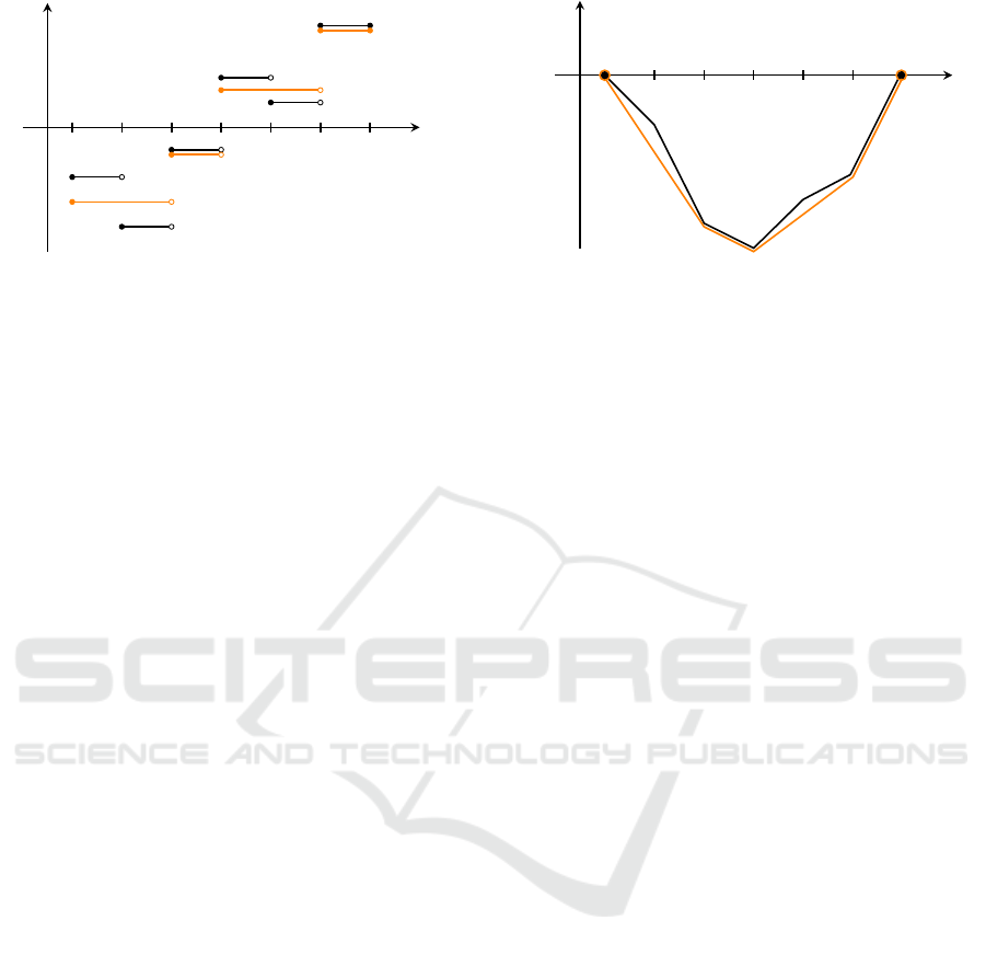
x
y
f
u
↑
= W
0
↑
a
b
(a) The piecewise constant input signal f and the mono-
tonic solution u
↑
to the isotonic regression problem.
x
y
a b
F
W
↑
(b) The cumulative signal F and the corresponding
lower convex envelope (or taut string) W
↑
.
Figure 2: A graphical illustrations of the taut string interpretation of isotonic regression.
Proposition 6 how application of the ROF model to
a piecewise constant signal leads to a piecewise con-
stant denoised signal with the same nodes (i.e. the
model is “edge-preserving”). This observation, toget-
her with the semi-group property, immediately sug-
gests a (perhaps not so efficient) non-iterative algo-
rithm for the computation of the denoising of a piece-
wise constant signal which is different from the one
in (Condat, 2013). If very fast non-iterative schemes
for finding the solution to the one-dimensional ROF
model can be devised then, as already indicated by L.
Condat, efficient iterative algorithms for image denoi-
sing using the two-dimensional ROF model (with the
‘Manhattan metric’ as measure of the image gradient
magnitude) may be constructed as well. We hope to
return to this topic in the future.
ACKNOWLEDGEMENTS
The author whishes to thank Viktor Larsson at the
Centre for Mathematical Sciences, Lund University,
for reading and commenting on several drafts of this
paper.
REFERENCES
Ambrosio, L., Fusco, N., and Pallara, D. (2000). Functi-
ons of Bounded Variation and Free Discontinuity Pro-
blems. Clarendon Press, Oxford.
Anevski, D. and Soulier, P. (2011). Monotone spectral den-
sity estimation. Ann. Statistics, 39:418–438.
Attouch, H., Buttazzo, G., and Michaille, G. (2015). Vari-
ational Analysis in Sobolec and BV Spaces; Applica-
tions to PDEs and Optimization. SIAM, New York,
2nd edition.
Br
´
ezis, H. (1999). Analyse fonctionelle—Th
´
eorie et appli-
cations. Dunod, Paris.
Chambolle, A. (2004). An algorithm for total variation mi-
nimization and applications. J. Math. Imaging Vis.,
20:89–97.
Condat, L. (2013). A direct algorithm for 1d total variation
denoising. IEEE Signal Proc. Letters, 20(11):1054–
1057.
Davies, P. and Kovac, A. (2001). Local extremes, runs,
strings and multiresolution. Annals of Statistics, 29:1–
65.
D
¨
umbgen, L. and Kovac, A. (2009). Extension of smoo-
thing via taut strings. Electronic Journal of Statistics,
3:41–75.
Gigli, N. and Mosconi, S. (2015). The abstract lewy-
stampacchia inequality and applications. J. Math. Pu-
res Appl., 104:258–275.
Grassmair, M. (2007). The equivalence of the taut string
algorithm and BV-regularization. J. Math. Imaging
Vis., 27:56–66.
Hinterberger, W. and Scherzer, O. (2006). Variational met-
hods on the space of functions of bounded Hessian for
convexification and denoising. Computing, 76:109–
133.
Hinterm
¨
uller, W. and Kunisch, K. (2004). Total bounded va-
riation regularization as a bilaterally constrained opti-
mization problem. SIAM J. Appl. Math., 64(4):1311–
1333.
Lewy, H. and Stampacchia, G. (1970). On the smoothness
of superharmonics which solve a minimum problem.
J. Analyse Math., 23:227–236.
Mammen, E. and van de Geer, S. (1997). Locally adaptive
regression splines. Annals of Statistics, 25(1):387–
413.
Meyer, Y. (2000). Oscillating Patterns in Image Processing
and Nonlinear Evolution Equations. American Mat-
hematical Society, New York.
Overgaard, N. C. (2017). On the taut string interpretation of
the one-dimensional Rudin-Osher-Fatemi model: A
new proof, a fundamental estimate and some appli-
cations. arXiv:1710.10985 [eess.IV]:1–19.
Rudin, L., Osher, S., and Fatemi, E. (1992). Nonlinear total
variation based noise removal algorithms. Physica D,
60:259–268.
Rudin, W. (1986). Real and Complex Analysis. McGraw-
Hill, New York, 3rd edition.
ICPRAM 2018 - 7th International Conference on Pattern Recognition Applications and Methods
242

Scherzer, O., Grasmair, M., Grossauer, H., Haltmeier, M.,
and Lenzen, F. (2009). Variational Methods in Ima-
ging. Springer, New York.
Setterqvist, E. (2016). Taut strings and real interpolation.
Linkoping Studies in Science and Technology Disser-
tations, 1801.
Zhu, M., Wright, S., and Chan, T. (2007). Duality-based
algorithms for total variation image restoration. Com-
put. Optim. Appl., 47:377–400.
APPENDIX A
As promised in the introduction, we are going to
prove that the solution of the minimization problem
(2) in STEP 3 of the Taut string algorithm coincides
with the solution of the shortest path problem (3). In
fact we prove the slightly more general statement:
Proposition. Let H denote any strictly convex C
1
-
function defined on R and set
L
H
(W ) =
Z
I
H(W
0
(x))dx .
Then the problem min
W ∈T
λ
L
H
(W ) has precisely
the same solution as the minimization problem
min
W ∈T
λ
E(W ) in (2).
The case we need in our analysis follows by taking
H(s) = (1 + s
2
)
1/2
.
Proof. The idea of the proof is to verify that W
λ
:=
argmin
W ∈T
λ
E(W ) solves the variational inequality:
Z
I
h(W
0
λ
(x))(W
0
(x) −W
λ
(x)
0
)dx ≥ 0 , for all W ∈ T
λ
,
(20)
where h = H
0
. This condition is both necessary and
sufficient for W
λ
to be a minimizer of L
H
over T
λ
,
and since L
H
is a strictly convex functional, there is
at most one such minimizer.
Being the minimizer of E over T
λ
, W
λ
∈ T
λ
satis-
fies the variational inequality (which is a special case
of (20) if we take H(s) = s):
Z
I
W
0
λ
(W
0
−W
0
λ
)dx ≥ 0, for all W ∈ T
λ
. (21)
Set C
+
= {x ∈ I : W
λ
(x) = F(x) + λ} and C
−
= {x ∈
I : W
λ
(x) = F(x) − λ}. These are the sets where the
solution touches the upper and the lower obstacles,
respectively. Since F and W
λ
are continuous, both sets
are closed. In fact, C
+
and C
−
are compact because
λ > 0 implies that they do not reach the boundary of
I. They are disjoint, C
+
∩ C
−
=
/
0, and their union,
C = C
+
∪C
−
, is the contact set for W
λ
.
For any non-negative ξ ∈ C
1
0
(I\C
+
) there exists an
ε > 0 such that W := W
λ
+ εξ belongs to T
λ
. If this W
is substituted into (21) we find that
Z
I
W
0
λ
ξ
0
dx ≥ 0 for all ξ ∈ C
1
0
(I\C
+
) with ξ ≥ 0.
It follows that −W
00
λ
is a positive measure on I\C
+
,
hence −W
0
λ
is non-decreasing on each connected
component of I\C
+
. Similarly one proves that −W
0
λ
is non-increasing on each connected component of
I\C
−
. This means, in particular, that W
0
λ
constant on
each connected component of I\C.
Since h is non-decreasing, the composite function
−h(W
0
λ
) has the same monotonicity properties as
−W
0
λ
. Therefore the distributional derivative −h(W
0
λ
)
0
is a positive measure µ
+
on I\C
+
and minus a posi-
tive measure −µ
−
on I\C
−
. Clearly supp µ
+
⊂ C
−
and supp µ
−
⊂ C
+
, so −h(W
0
λ
)
0
is a signed measure µ
with the Jordan decomposition µ = µ
+
− µ
−
. The fol-
lowing calculation now verifies (20): For any W ∈ T
λ
we have
Z
I
h(W
0
λ
)(W
0
−W
0
λ
)dx = −
Z
I
W −W
λ
dµ
= −
Z
I
W −W
λ
dµ
+
+
Z
I
W −W
λ
dµ
−
≥ 0
which holds because W − W
λ
≥ 0 on C
−
and W −
W
λ
≤ 0 on C
+
.
APPENDIX B
We prove the inequality (16) used in the proof of The-
orem 2. With the notation introduced in this proof we
can formulate this result as follows:
Proposition (Lewy–Stampacchia inequality). Sup-
pose φ
00
and ψ
00
are signed measures. Then the mi-
nimizer u
0
of E over C = {u : φ ≤ u ≤ ψ} satisfies
−(φ
00
)
−
≤ u
00
0
≤ (ψ
00
)
+
where µ
+
and µ
−
denote the positive and negative va-
riations, respectively, of the signed measure µ.
Note that the functional E is defined, convex and
differentiable on H
1
(I) and therefore satisfies the in-
equality
E(v) − E(u) ≥
Z
b
a
u
0
(x)(v
0
(x) − u
0
(x))dx, (22)
for all u,v ∈ H
1
(I), as is easily checked. We also
know that min
C
E has a unique solution u
0
∈ C (use
the projection theorem) which satisfies the necessary
and sufficien condition:
Z
b
a
u
0
0
(v
0
− u
0
0
)dx ≥ 0 for all v ∈ C.
On the Taut String Interpretation of the One-dimensional Rudin–Osher–Fatemi Model
243

Proposition 8 was first proved for the unilateral
obstacle problem (in multiple dimensions) in (Lewy
and Stampacchia, 1970) and since extended to bilate-
ral obstacle problems. Here we present a proof based
on the sub-modularity of the functional E, that is, for
all u,v ∈ H
1
(I),
E(u ∧ v) + E(u ∨ v) ≤ E(u)+ E(v), (23)
where u ∧ v := max(u, v) and u ∨ v := min(u, v) both
belong to H
1
(I). In fact, the functional E is so sim-
ple that equality holds for all u,v. This method of
proof was invented recently by (Gigli and Mosconi,
2015) and used to prove a very general version of the
bilateral Lewy–Stampacchia inequality. We use their
approach.
Proof. We prove the rightmost inequality, u
00
0
≤
(ψ
00
)
+
, the leftmost one then follows by a symme-
try argument: −u
0
minimizes E over the −C = {u ∈
H
1
0
(I) : −ψ ≤ u ≤ −φ}.
To simplify notation we set ψ
00
= µ. Define the
new functional
ˆ
E(u) = E(u) + hµ
+
,ui and consider
the minimization problem
min
u∈H
1
0
(I):u≥u
0
ˆ
E(u). (24)
The goal is to prove that u
0
itself solves this problem.
This will imply the desired inequality, as we shall see
below.
First the following claim is proved: For any u ∈
H
1
0
(I) satisfying u ≥ u
0
we have
ˆ
E(u ∧ ψ) ≤
ˆ
E(u). (25)
Since ψ > 0 on ∂I and u ∈ H
1
0
(I) we get u∧ψ ∈ H
1
0
(I)
which is therefore admissible for the min-problem
above. The claim is proved using the sub-modularity
(23) of E and the identity u ∧ v + u ∨ v = u + v with v
replaced by ψ:
ˆ
E(u) −
ˆ
E(u ∧ ψ)
= E(u) − E(u ∧ ψ) + hµ
+
,u − u ∧ ψi
≥ E(u ∨ ψ) − E(ψ) + hµ
+
,u ∨ ψ − ψi
≥ E(u ∨ ψ) − E(ψ) + hψ
00
,u ∨ ψ − ψi
≥ E(u ∨ ψ) − E(ψ) − hψ
0
,(u ∨ ψ)
0
− ψ
0
i ≥ 0,
where the last inequality follows from (22).
The claim (25) shows that the minimum of
ˆ
E over
{u ≥ u
0
} coincides with the minimum over {ψ ≥ u ≥
u
0
}. Therefore, since u − u
0
≥ 0, we find
ˆ
E(u) −
ˆ
E(u
0
) = E(u) − E(u
0
) + hµ
+
,u − u
0
i
≥ E(u) − E(u
0
) ≥ 0,
where the last estimate follows from the observation
that {u : u
0
≤ u ≤ ψ} ⊂ C and that u
0
minimizes E
over C. That is, u
0
is the solution of (24).
The necessary condition for u
0
to be a minimizer
for
ˆ
E reads:
d
dα
ˆ
E((1 − α)u
0
+ αu)
α=0
≥ 0
for all u ∈ H
1
0
(1) satisfying u ≥ u
0
. That is,
Z
b
a
u
0
0
(u
0
− u
0
0
)dx + hµ
+
,u − u
0
i ≥ 0
for all u ∈ H
1
0
(I) satisfying u ≥ u
0
. This implies
h−u
00
0
+ µ
+
,ϕi ≥ 0 for all ϕ ∈ C
1
0
(I) such that ϕ ≥ 0
on I. Therefore −u
00
0
+µ
+
is a positive measure, hence
u
00
0
≤ µ
+
, which is the desired result.
ICPRAM 2018 - 7th International Conference on Pattern Recognition Applications and Methods
244
