Using Goal Programming on Estimated Pareto Fronts to Solve

Multiobjective Problems

Rodrigo Lankaites Pinheiro

1,2

, Dario Landa-Silva

, Wasakorn Laesanklang

and Ademir Aparecido Constantino

Webroster Ltd., PE1 5NB, Peterborough, U.K.

ASAP Research Group, School of Computer Science, The University of Nottingham, U.K.

Department of Mathematics, Faculty of Science, Mahidol University, Thailand

Departamento de Inform

atica, Universidade Estadual de Maring

a, Maring

a, Brazil

Keywords:

Multi-criteria Decision Making, Goal Programming, Pareto Optimisation.

Abstract:

Modern multiobjective algorithms can be computationally inefﬁcient in producing good approximation sets

for highly constrained many-objective problems. Such problems are common in real-world applications where

decision-makers need to assess multiple conﬂicting objectives. Also, different instances of real-world pro-

blems often share similar ﬁtness landscapes because key parts of the data are the same across these instances.

We we propose a novel methodology that consists of solving one instance of a given problem scenario using

computationally expensive multiobjective algorithms to obtain a good approximation set and then using Goal

Programming with efﬁcient single-objective algorithms to solve other instances of the same problem scena-

rio. We propose three goal-based objective functions and show that on a real-world home healthcare planning

problem the methodology can produce improved results in a shorter computation time.

1 INTRODUCTION

Modern multiobjective algorithms struggle to ﬁnd

good approximation sets on highly constrained pro-

blems or when the number of objectives is high Gi-

agkiozis and Fleming (2012). Decision-makers of-

ten require a single solution and the Pareto front is

only useful to enable them to choose the preferred so-

lution(s). There are a few techniques that use dom-

ain knowledge to estimate Pareto fronts. Giagkio-

zis and Fleming (2014) propose a technique to es-

timate the Pareto front of continuous multiobjective

problems and then use the estimated front to obtain

values for the decision variables of interesting soluti-

ons. Their technique is particularly useful because it

can be applied to subregions of the objective space.

Another technique is Bayesian multiobjective optimi-

sation, which consists of using a Bayesian model to

learn computationally expensive objective functions

and use the estimation model to quickly explore the

search space Feliot et al. (2016).

In this research we tackle a workforce scheduling

and routing problem (WSRP). A WSRP solution is a

plan in which skilled mobile workers are scheduled to

visit locations that are geographically scattered. Real-

world applications of WSRP usually involve multiple

objectives. However, most approaches in the litera-

ture tackle this problem using a weighted sum to com-

bine the multiple objectives into one. Even genera-

ting single-objective solutions for the WSRP has been

shown to be difﬁcult for problem instances of consi-

derable size Castillo-Salazar et al. (2014, 2016); Lae-

sanklang et al. (2015a). The WSRP arises in several

domains, for example when scheduling home healt-

hcare workers, technicians, and security personnel

among others. Here, we consider the problem of sche-

duling nurses and care workers to visit and provide

care services to patients in their homes. Works in the

literature tackling home healthcare planning problems

usually use data from real-world scenarios Fikar and

Hirsch (2017). This is also the case in the present

work. We employ data from six distinct home healt-

hcare scenarios provided by Webroster Ltd., who pro-

vides enterprise resource planning software for home

healthcare companies.

The quality of solutions to the WSRP considered

here can be measured using several criteria like: in-

curred costs, travel distance, satisfaction of staff pre-

132

Pinheiro, R., Landa-Silva, D., Laesanklang, W. and Constantino, A.

Using Goal Programming on Estimated Pareto Fronts to Solve Multiobjective Problems.

DOI: 10.5220/0006718901320143

In Proceedings of the 7th International Conference on Operations Research and Enterprise Systems (ICORES 2018), pages 132-143

ISBN: 978-989-758-285-1

ferences, satisfaction of patients preferences, etc. Due

to the high number of constraints and objectives in

this problem, even state-of-the-art multiobjective al-

gorithms struggle to ﬁnd good approximations to the

Pareto front within reasonable computation time. In

problems like this where each instance is a repetition

of the same situation but in different days, parts of

the data repeat across multiple instances of the same

problem scenario. For example, the same set of staff

is available for different days with only minor chan-

ges regarding staff avilability. Also, there is a set of

recurring visits that need to be scheduled in each in-

stance of the problem scenario. This happens in other

problems like vehicle routing and nurse scheduling

where instances of the same problem scenario exhi-

bit similar ﬁtness landscapes (η-dimensional surface

representing the Pareto front, where η is the number

of objectives). This issue was investigated in Pinheiro

et al. (2015, 2017) which proposed a technique to ana-

lyse and visualise complex objective relationships and

ﬁtness landscapes in multiobjective problems. Thus,

this paper proposes a methodology that exploits this

similarity between instances of a multiobjetive opti-

misaton problem, in order to solve instances of the

problem more efﬁciently.

The proposed methodology works as follows. For

a given dataset consisting of multiple instances of the

problem scenario, a single pilot instance is solved

using multiobjective algorithms or the best available

method in order to produce an approximation to the

Pareto optimal set. A decision-maker uses this ap-

proximation set to choose target solutions for the re-

maining instances of the dataset. The chosen target

solutions represent the desired trade-off between the

multiple objectives. Then, goal programming is app-

lied with an efﬁcient single-objective solving method

to obtain solutions that in quality are close enough to

(or better than) the chosen target solutions. Hence,

the main contributions of this work are:

1. A novel methodology that employs an approxi-

mation to the Pareto optimal front of a pilot pro-

blem instance, to solve other similar instances of

the same problem with goal programming and ef-

ﬁcient single-objective algorithms.

2. The assessment of three approaches to deﬁne the

goal programming objective function, one uses

a Chebyshev objective function, another uses a

weighted function derived from the target solu-

tion, and the third one uses an objective function

that seeks to minimise the largest deviation to ob-

jective values in the target solution.

The remaining of this paper is structured as fol-

lows. Section 2 outlines the Workforce Schedu-

ling and Routing Problems Project, which is used

to illustrate the application of the proposed metho-

dology. Section 3 presents the proposed methodo-

logy. Section 4 presents the experimental conﬁgu-

ration while section 5 presents the results. Finally,

section 7 concludes this work.

2 THE WORKFORCE

SCHEDULING AND ROUTING

PROBLEM

The WSRP is an optimisation problem that combines

a scheduling and a routing problem. A set of m wor-

kers {w

,... ,w

}, must perform tasks on a set of

n visits {v

,. .. ,v

}, which are distributed across

distinct geographical locations. This work considers

a speciﬁc case of this problem: the home healthcare

planning problem, where workers are nurses, doctors

and care workers and the purpose of the visits is to

provide care to patients in their homes. For more in-

formation about this WSRP, please refer to Castillo-

Salazar et al. (2012, 2016).

The WSRP studied in this work contemplates the

planning of a single day. Several hard constraints are

considered in the problem: visits require a set of skills

and only workers possessing the required skills can be

assigned; workers can only be assigned to visits if al-

lowed by their respective contracts; every visit must

commence at a speciﬁed time in which workers must

already be at the visits’ premises; no time clashes are

allowed, i.e. a worker cannot be assigned to simulta-

neous visits and there must be enough time for a wor-

ker to travel between visits. Also, two soft constraints

are considered: workers may have a list of time inter-

vals in which they are available; locations are grouped

by geographical areas and workers may have a list of

areas in which they are available.

The objectives considered in the problem are:

denotes the sum of the distances travelled by the

workers, including commuting from their home

to the ﬁrst assignment, between each assignment,

and from the ﬁnal assignment back to their home;

denotes the sum of monetary assignment costs

(workers wages for the assigned visits);

denotes the sum of skill preferences in respect of

assigning workers with skills that are desirable but

not necessary;

denotes the sum of patients preferences in respect

of assigning preferred workers; and

denotes the sum of workers preferences in respect

of assigning workers to visits in their preferred

area.

Using Goal Programming on Estimated Pareto Fronts to Solve Multiobjective Problems

133

(a) Instance B1 (b) Instance B3 (c) Instance B5

(d) Instance D2 (e) Instance D4 (f) Instance D6

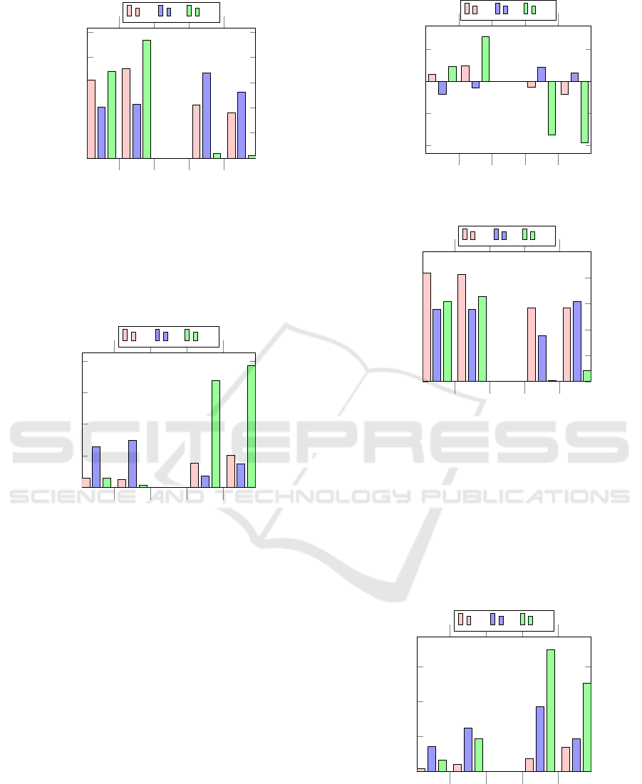
Figure 1: Scatter plots of three instances of datasets B and D. In each case, the x axis shows the value of objective Z

and the

y axis shows the values of each of the other objectives in different colours.

Data from four different home healthcare compa-

nies of different sizes and characteristics was provi-

ded and six problem scenarios or dataset were gene-

rated. Each dataset (A, B, C, D, E and F) is composed

of 7 instances for a total of 42 problem instances. Set

A has small instances (number of visits and workers)

while set F has the largest instances.

Other works in the literature have also tackled the

WSRP datasets considered here:

• Laesanklang et al. (2015a) presented a computa-

tional study on the suitability of using exact met-

hods to solve the problem. It was concluded that

only the smaller instances can be solved to opti-

mality by a mathematical solver. Later, Laesan-

klang et al. (2015b) proposed to decompose the

problem by geographical locations in order to em-

ploy the mathematical solver on the sub-problems

and then use heuristic algorithms to integrate the

partial solutions.

• Algethami and Landa-Silva (2015) conducted a

study of various genetic operators applied to this

problem. It was observed that the high number of

constraints and large size of the instances presen-

ted a considerable challenge to the standard ge-

netic algorithm implemented. Later, Algethami

et al. (2016) proposed a knowledge-based indirect

representation and genetic operators to improve

the efﬁciency of the genetic algorithm for tackling

the problem.

• More recently, Pinheiro et al. (2016) presented a

Variable Neighbourhood Search (VNS) metaheu-

ristic to tackle the WSRP, incorporating two no-

vel heuristics tailored to the problem-domain. The

ﬁrst heuristic restricts the search space using a pri-

ority list of candidate workers and the second heu-

ristic seeks to reduce the violation of speciﬁc soft

constraints. Also, two greedy constructive heuris-

tics were used to give the VNS a good starting

point. Since that VNS is the best-known algo-

rithm to tackle these WSRP instances, that algo-

rithm is employed here within the proposed goal

programming framework.

As preliminary work, we applied the analysis

technique proposed by Pinheiro et al. (2015, 2017) on

all instances considered here. The technique consists

of performing four steps: ﬁrst the global pairwise re-

lationships are analysed using the Kendall correlation

method; then the ranges of the values found on the gi-

ven approximation front are estimated and assessed;

next these ranges are used to plot a map using Gray

code, similar to Karnaugh maps, that has the ability

to highlight the trade-offs between multiple objecti-

ves; and ﬁnally local relationships are identiﬁed using

scatter plots. The conclusion is that in the studied da-

tasets, instances of the same datset indeed present si-

milar ﬁtness landscapes. Figure 1 provides evidence

of that and shows the scatter plots of instances B-01,

B-03, B-05, D-02, D-04, and D-06 (arbitrarily cho-

sen). Each datapoint corresponds to normalised ob-

jective values. For reasons of space, we omit the other

datasets and the scatter plots of all instances. The re-

semblance between the ﬁtness landscapes of the pre-

sented instances of datasets B and D is evident. Also,

it is clear that different datasets present distinct ﬁtness

ICORES 2018 - 7th International Conference on Operations Research and Enterprise Systems

134

landscapes, even though they correspond to the same

problem formulation. Finally, it is important to emp-

hasise that datasets A, B and C present similar ﬁtness

landscapes with solutions well spread throughout the

objective space while datasets D, E and F present dis-

tinct ﬁtness landscapes with complex objective relati-

onships and gaps.

3 PROPOSED METHODOLOGY

Figure 2 presents the overall concept of the proposed

methodology. We use the aforementioned WSRP to

illustrate the concept. Following, we explain each of

the four numbered steps indicated.

Figure 2: Overview of the proposed methodology. The

numbered steps are explained below.

1. A pilot instance within the dataset is selected

by the decision-maker and solved using multiob-

jective algorithms to obtain the best possible non-

dominated approximation set. The pilot instance

must be representative and present similar featu-

res to other instances.

2. The decision-maker chooses an appropriate solu-

tion t from the obtained non-dominated set. This

chosen solution is known as the target solution

and its objective-vector is denoted by

= (Z

3. Each remaining instance in the dataset may now

be solved by the VNS (Pinheiro et al., 2016) using

a modiﬁed objective function (goal programming

variant) that attempts to reach the target objective

vector in the current dataset.

4. The ﬁnal solution obtained by the modiﬁed VNS

is presented.

The modiﬁed objective function of step 3 has

an important role in the methodology. Following,

we present three approaches for determining the ob-

jective function. The ﬁrst is the well known Cheby-

shev approach. The second aims to derive a weight-

vector from the target solution and the approximation

set of the pilot instance. The third approach mini-

mises the Euclidean distances to the target objective-

vector.

3.1 Chebyshev Goal Programming

Chebyshev goal programming (Flavell, 1976) is one

of the most widely employed goal programming

techniques that does not necessarily rely on the deci-

sion maker to set priorities between objectives (Jones

and Tamiz, 2016). The technique aims to obtain a ba-

lanced solution by minimising the gap to the target of

the objective that presents the highest gap. Hence, if

the target goals for the objectives are similarly difﬁ-

cult to be reached, the Chebychev GP technique can

obtain a balanced solution. However, if at least one

target objective value is more difﬁcult to achieve (i.e.

the target goal is too optimistic), the quality of that

objective can be a bottleneck for the remaining ob-

jectives because the search will solely focus on im-

proving that objective. We deﬁne the Chebyshev ob-

jective function for the WSRP as follows:

Minimise λ (1)

Subject to

≤ λ (2)

≤ λ (3)

≤ λ (4)

≤ λ (5)

≤ λ (6)

The Chebyshev objective function given by Eq.

(1) is used as the objective function for the WSRP.

The main objective is now to minimise λ, thus ﬁn-

ding a well-balanced solution regarding reaching the

target values. If all targets are reached, λ can assume

fractional values and a solution that shows balanced

improvements on all objectives may be obtained.

Using Goal Programming on Estimated Pareto Fronts to Solve Multiobjective Problems

135

3.2 Derived Weight Vector

One problem with the Chebyshev approach is that it

does not guarantee Pareto efﬁciency. However, the

optimal solution of a weighted sum (where weights

are not simultaneously null) objective function is al-

ways Pareto efﬁcient. To derive a weight vector from

the target solution, we ﬁrst convert the approxima-

tion set of the pilot instance into a system of linear

inequalities. Considering that the approximation set

is composed of n objective-vectors (

, .. .,

the linear inequalities system can be deﬁned as fol-

lows where the aim is to determine the values of

~w = (w











≤ ~w

(7)

There is no guarantee that the system of linear in-

equalities has a solution because the ﬁtness landscape

is non-convex, meaning that no set of weights can be

set to achieve some points in the front. Therefore,

instead of ﬁnding a solution for the system, we aim to

ﬁnd a weight vector ~w that satisﬁes the largest num-

ber of inequalities. Hence, we deﬁne the problem of

ﬁnding the best weight vector as the following MIP

(mixed-integer programming) minimisation problem.

Minimise

∑

j=1

(8)

subject to

−~w

≤ Mx

, j = 1,. .. ,n (9)

∈ (0, 1], x

binary ,

(

i = 1, .. ., 5

j = 1, .. ., n

(10)

Note that M is a very large constant.

The objective function given by Eq. (8) aims to

ﬁnd a weight vector ~w that minimises the number of

linear inequalities in the system (7) which do not ful-

ﬁll the condition ~w

≤ ~w

expressed by constraint

(9). Note that constraint (10) guarantees that zero can-

not be chosen as a weight-value as we do not want

criteria to be removed.

Finally, the weight vector ~w obtained from the

MIP model is used in the objective function for the

WSRP as given by Eq. (11).

Minimise

∑

i=1

(11)

3.3 Euclidean Distances

We propose an alternative based on the Euclidean dis-

tances to the target vector. In essence, this is a met-

hod that considers all objectives as equally impor-

tant. Hence, minimising the Euclidean distances al-

one does not guarantee Pareto efﬁciency. In order to

reduce this issue, the proposed method consists of mi-

nimising the distances to the target vector for the ob-

jectives that are worse than the target. If the current

distance for the objectives that are worse than the tar-

get vector is small (< ε), then the aim is to maximise

the distances of the objectives that are better than the

target vector.

Henceforth, the objective function in Eq. (12) be-

comes the objective function for the WSRP.

Minimize

(

z ,if z > ε

−z

,otherwise

(12)

where

z =

∑

i=1

(13)

∑

i=1

(14)

(

− Z

)

,if Z

> Z

0 ,otherwise

(15)

(

− Z

)

,if Z

≤ Z

0 ,otherwise

(16)

In summary, when the Euclidean distances of the

objectives that are worse than the target vector are lar-

ger than the given parameter ε, the objective function

consists of minimising the Euclidean distances (z).

Otherwise, when z ≤ ε, the objective consists of max-

imising the distances for the objectives that are better

than the target solution (z

). Thus, if the solution has

not reached the target, the objective function attempts

to close the gap to the target. If the solution is close or

better than the target, the objective function attempts

to further improve it.

ICORES 2018 - 7th International Conference on Operations Research and Enterprise Systems

136

4 EXPERIMENTAL

CONFIGURATION

We applied the proposed methodology to the WSRP

datasets mentioned previously. The ﬁrst instance of

each dataset (A-01, B-01, C-01, D-01, E-01 and F-

01) was selected as the pilot instance of its respective

dataset. We used the approximation sets obtained as

described next. Fifteen target vectors were randomly

selected (uniformly distributed) from each approxi-

mation set and the same target vectors were used for

the Derived Weight Vector (WV) objective function,

the Euclidean Distances (ED) objective function, and

the Chebyshev (CV) objective function.

For each remaining instance in each dataset,

the Full-VNS algorithm proposed by Pinheiro et al.

(2016) was applied to the ﬁfteen selected target vec-

tors from the pilot instance of its respective dataset

using all three objective functions. For each target

vector of each instance, we ran the Full-VNS algo-

rithm eight times for one minute each. The results

shown comprise the aggregate data.

Multiobjective algorithms struggle to ﬁnd good

approximation sets in combinatorial problems with

many objectives (more than three) (Giagkiozis and

Fleming, 2012). Hence, we resort to a tailored pro-

cedure to obtain an improved approximation set. Gi-

agkiozis and Fleming (2014) state that most multiob-

jective algorithms can be classiﬁed as either Pareto-

based or decomposition-based. This study utilises

NSGA-II (Deb et al., 2002) as the Pareto-based al-

gorithm and MOEA/D (Zhang and Li, 2007) as the

decomposition-based. Thus, for each problem in-

stance the approximation set was obtained as follows:

1. run both the NSGA-II and MOEA/D for one mil-

lion objective evaluations on each possible bi-

objective vector (Z

, Z

), (Z

, Z

), .. . (Z

, Z

);

2. run both the NSGA-II and MOEA/D for one mil-

lion objective evaluations on each possible three-

objective vector (Z

, Z

), (Z

, Z

), . .. (Z

, Z

);

3. run both the NSGA-II and MOEA/D for one mil-

lion objective evaluations on each possible four-

objective vector (Z

, Z

), (Z

, Z

.. . (Z

, Z

);

4. create an archive composed of the non-dominated

solutions found in the previous three steps;

5. generate a population of individuals where half of

the elements are randomly generated and the other

half are randomly drawn from the archive built in

the previous step;

6. run both the NSGA-II and MOEA/D four times

each, for two million objective evaluations, using

the initial population generated in the previous

step and the ﬁve-objective vector; and

7. compile an approximation set with all non-

dominated solutions found in all steps.

The number of solution vectors obtained for each

pilot instance was as follows: 1162 for A-01, 1302

for B-01, 1830 for C-01, 2470 for D-01, 3689 for E-

01 and 1500 for F-01.

5 EXPERIMENTAL RESULTS

First, we show the effectiveness of the derived weight

vector obtained from the MIP model presented in Eq.

(8)–(10). The effectiveness of a weight vector ~w is

given by the percentage of solutions (in the pilot in-

stance of the approximation set) in which ~w

≤ ~w

i = 1,. .. ,5. Hence, if the effectiveness is 100%, it

means that the MIP model found a solution for the

inequalities system in Eq. (7).

A-01 B-01 C-01 D-01 E-01 F-01

90%

92%

94%

96%

98%

100%

Dataset

Weigth Vector Effectiveness

Figure 3: Average percentage of the solutions in the approx-

imation set of each target instance such that ~w

≤ ~w

Figure 3 presents the results of the effectiveness

analysis of the weight vectors obtained. In all pilot in-

stances, the effectiveness surpassed 90% on average.

Pilot instance D-01 presented the worst overall ef-

fectiveness, with an average of 93.5%, while pilot in-

stance A-01 presented the most effective weight vec-

tors averaging 99.5%. In all cases, the MIP model

provided good weight vectors and these were applied

to the WV objective function in Eq. (8).

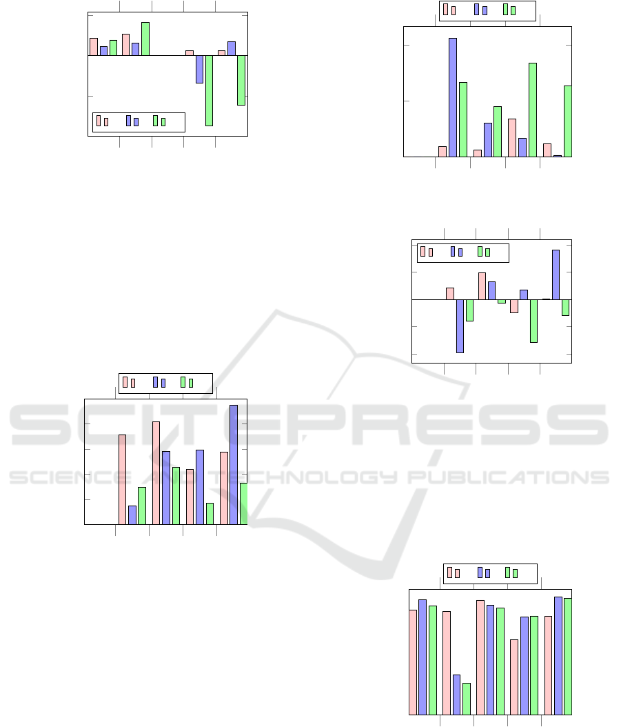
Next, we show the results for each dataset in three

charts. The target achievement chart displays the per-

centage of solutions, in the given dataset, that achie-

ved the target value in each objective. The gap to tar-

get chart contains the average gap to the target so-

lutions for the solutions that did not reach the tar-

get. Finally, the overall comparison chart displays the

average quality of solutions where positive values in-

dicate that, on average, the solutions found are better

than the target solution and negative values indicate

that the solutions are worse than the target solution.

Using Goal Programming on Estimated Pareto Fronts to Solve Multiobjective Problems

137

20%

40%

60%

80%

100%

WV ED

Figure 4: Dataset A – target achievement.

Figures 4–6 present the results of applying the

VNS algorithm with the WV, ED and CV objective

functions to the remaining instances of dataset A. Re-

sults comprise the average values of eight runs for

each target vector of each problem instance for each

objective function.

10%

20%

30%

40%

WV ED

Figure 5: Dataset A – gap to the target.

In Figure 4, the percentage of achievement of in-

dividual target objective is shown. Note that there are

no values for Z

because dataset A does not present

preferred skills information. It is clear that the CV ob-

jective function presented better overall target achie-

vement on Z

and Z

, followed by WV, while the ED

objective function is better on Z

and Z

, whilst CV

clearly underperforms.

Figure 5 shows that the average gap of the solu-

tions that did not reach the target is always smaller

than 16% for WV and ED, but high for CV. Also, in

conformity with the previous chart, the CV objective

function presented better values for the objectives Z

and Z

while the ED objective function obtained bet-

ter values for Z

and Z

. The CV objective function

presented large gaps on the two latter objectives. Fi-

nally, in Figure 6, it is clear that on average solutions

are at most 10% off the target for WV and ED, but

the CV approach clearly presents a stronger bias to-

wards Z

and Z

causing the quality of Z

and Z

deteriorate.

−40%

−20%

20%

WV ED

Figure 6: Dataset A – overall comparison.

20%

40%

60%

80%

100%

WV ED

Figure 7: Dataset B – target achievement.

The results for dataset B are presented in Figures

7–9. In Figure 7, it is clear that the WV objective

function obtains better target achievement than the

ED on Z

, Z

and Z

. On Z

the ED has a small advan-

tage. Also, when compared to dataset A, the average

overall achievement of the targets is higher for WV

and ED, but not for CV. The CV objective function

shows competitive results on Z

and Z

, but presents

extremely low achievement rates on Z

and Z

10%

20%

30%

WV ED

Figure 8: Dataset B – gap to the target.

Figure 8 shows that on all objectives, the WV ob-

jective function obtained smaller average gaps for the

solutions that have not met the target. Conversely, the

ICORES 2018 - 7th International Conference on Operations Research and Enterprise Systems

138

−20%

20%

WV ED

Figure 9: Dataset B – overall comparison.

CV objective function presents large gaps on Z

and

. Figure 9 displays that on average, the objective

function WV can provide improved objective-values

on all objectives. However, the objective function ED

presents improved results on Z

, Z

and Z

only, fai-

ling to deliver good results on Z

, while CV presents a

similar behaviour as on dataset A: good performance

on Z

and Z

but bad performance on Z

and Z

. Thus,

in this dataset, the WV objective function presents a

better alternative to solve the problem.

20%

40%

60%

80%

100%

WV ED

Figure 10: Dataset C – target achievement.

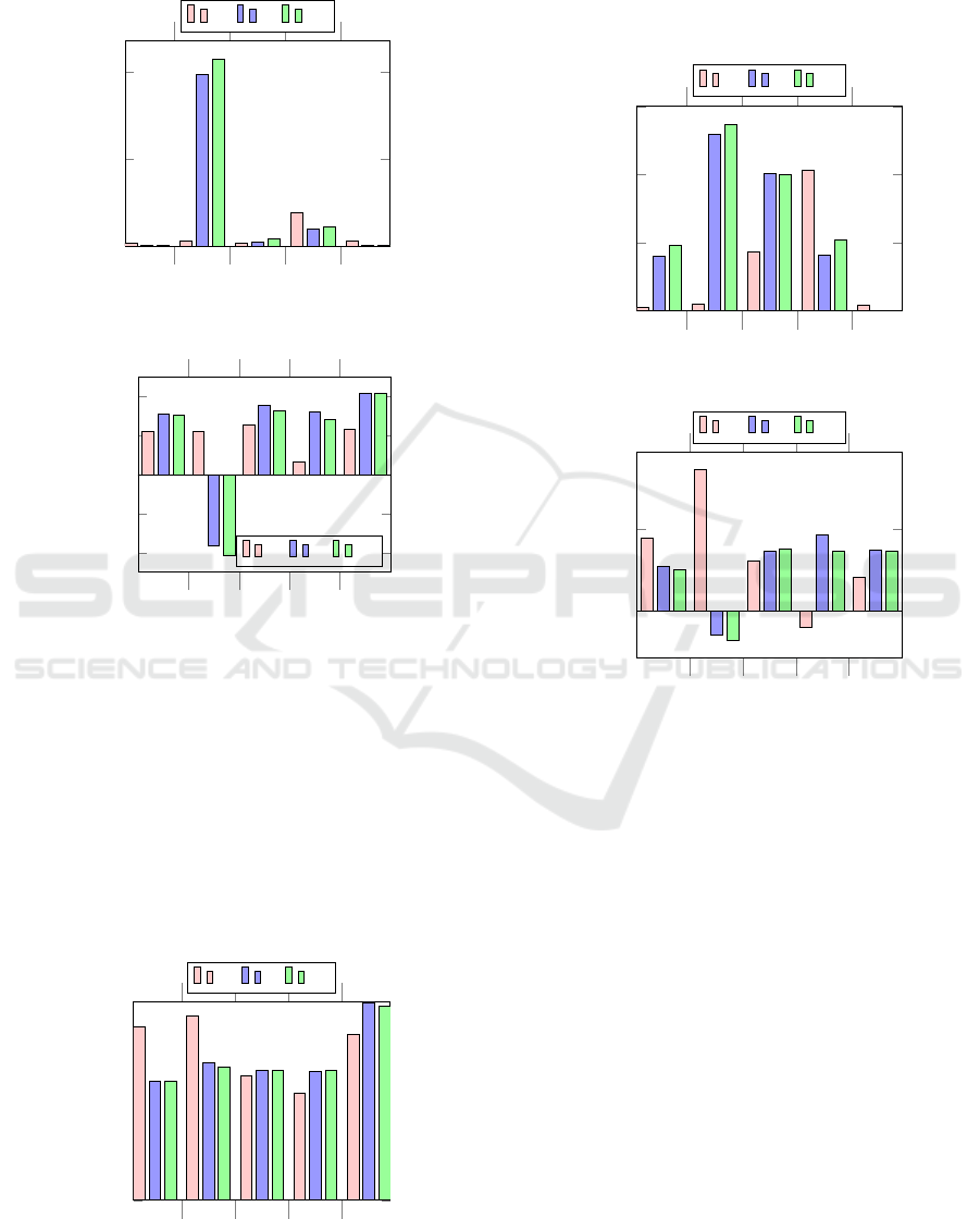
Figures 10–12 present the results for dataset C.

Note that since that dataset does not have distances in-

formation, Z

is always zero. In Figure 10, it is clear

both the objective functions WV and ED are balan-

ced, with WV presenting better results for Z

and Z

while the ED has the edge on Z

and Z

. However, the

ED objective function presents deteriorated results on

and exceptional results on Z

. The CV objective

function underperforms compared to the other met-

hods.

On Figure 11, it is clear that the ED objective

function not only struggles to reach the target for Z

but it also misses it by 40% on average. This infor-

mation is also reﬂected in Figure 12. Overall, the WV

objective function presents a more consistent choice

for this dataset as only on Z

the overall results are

negative and the average overall performance is su-

20%

40%

WV ED

Figure 11: Dataset C – gap to the target.

−40%

−20%

20%

40%

WV ED

Figure 12: Dataset C – overall comparison.

perior. Again, the CV objective function presents the

worst results as it can be seen that for every objective

there is a deﬁcit in the overall quality obtained.

Also, it is important to notice that this dataset pre-

sents a high variance in the sizes of the instances.

Therefore, because C-01 is a large instance, the tar-

get solution simply cannot be achieved on the smaller

instances of that dataset (C-02, C-04, C-05 and C-07).

20%

40%

60%

80%

100%

WV ED

Figure 13: Dataset D – target achievement.

The results for dataset D are presented by Figu-

res 13–15. In Figure 13 we see an overall increase on

the target achievement when compared to the previ-

ous datasets (A, B and C). As with dataset C, the ED

objective function displayed poor performance for Z

Using Goal Programming on Estimated Pareto Fronts to Solve Multiobjective Problems

139

but had better performance on three other objectives

, Z

and Z

). The CV objective function presented

competitive results on this dataset.

20%

40%

WV ED

Figure 14: Dataset D – gap to the target.

−40%

−20%

20%

40%

WV ED

Figure 15: Dataset D – overall comparison.

Figure 14 shows that, except for the ED and CV

objective functions on Z

, the gap for the solutions

that have not met the target is small. Also, except for

that objective, the overall average results (Figure 15)

show that all three objective functions present good

results, with the ED surpassing the WV on all ob-

jectives except on Z

and the CV presenting results

slightly worse than the ED. Still, the WV objective

function manages to present a higher consistency than

the other objective functions, and it also manages to

present good results for all objectives.

20%

40%

60%

80%

100%

WV ED

Figure 16: Dataset E – target achievement.

Dataset E results are presented in Figures 16–18.

Like with dataset D, a high overall target achievement

rate is shown (Figure 16). The WV objective function

present exceptional results on Z

and Z

, but fail to

beat the other objective functions on the remaining

objectives.

10%

15%

WV ED

Figure 17: Dataset E – gap to the target.

20%

WV ED

Figure 18: Dataset E – overall comparison.

It is clear from Figure 17 that the ED and CV

objective functions present higher gaps to the target

solutions. Figure 18 shows that all objective functi-

ons perform well on this dataset. The WV objective

function presents better performance on Z

and Z

while the ED objective function presents better results

on Z

. The CV objective function presents the best re-

sults on Z

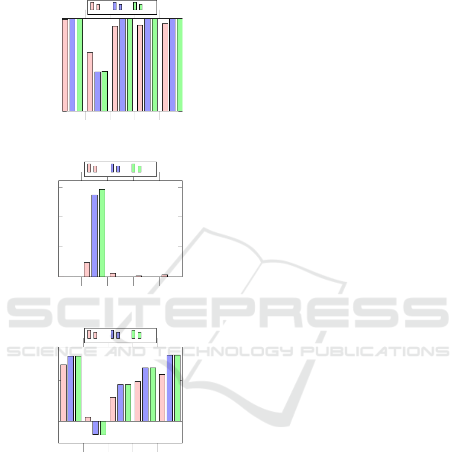
Lastly, the results for dataset F are presented in Fi-

gures 19–21. The target achievement rates (Figure 19)

show that all three objective functions perform well

on this dataset. However, on Z

the WV objective

function is noticeably better.

Figure 20 reinforces that claim as the gap for ob-

jective Z

is much larger for the ED and CV objective

functions. Finally, Figure 21 shows that on average,

the solutions provided by the WV objective function

are better than the target solutions for all objectives,

and, while the ED and CV objective functions present

better results than the WV on Z

, Z

and Z

, on Z

the average results are worse than the target values.

ICORES 2018 - 7th International Conference on Operations Research and Enterprise Systems

140

20%

40%

60%

80%

100%

WV ED

Figure 19: Dataset F – target achievement.

10%

20%

30%

WV ED

Figure 20: Dataset F – gap to the target.

50%

WV ED

Figure 21: Dataset F – overall comparison.

6 DISCUSSION

It was shown that both the WV (derived weighted vec-

tor) and ED (Euclidean distances) objective functions

provide good results on the majority of the scenarios,

with the WV objective function being slightly bet-

ter than the ED objective function on average. Also,

for the ﬁrst three scenarios, the CV objective function

clearly presented inferior results. It is noticeable that

the results were better on the largest datasets D, E and

F. In Section 2 we explained that the smallest datasets

are also the ones with solutions well spread throug-

hout the objective space. Also, it was mentioned that

datasets D, E and F present unique ﬁtness landsca-

pes with several regions containing no solutions and

several local relationships. Therefore, in the smal-

lest datasets, if the objective function is not accurate

enough (regarding reaching the target solution), the

search can deviate from the region of interest more

easily because the objective space is smoother. On the

largest datasets, because the objective space contains

gaps and local relationships, it may be enough for the

search (driven by the objective function) to reach the

same region as the target solution.

Take for instance the example in Figure 22. The

blue dots represent the Pareto front, the green dot is

the target solution, the red dot is the solution found by

the search and the yellow arrow is the search direction

given by the objective function. Note that the search

direction is not accurate, hence it does not point to-

wards the target solution (this is a valid assumption

given that we are either estimating the weight vector

or approximating the Euclidean distances). In Figure

22a, we have a well spread Pareto front and because

there exists a solution aligned with the search vector

(red dot), that solution is taken as the best solution. In

the given example, the chosen solution is better than

the target regarding the objective presented in the x

axis, but it is worse than the target regarding the ob-

jective represented by the y axis.

In Figure 22b, we have a Pareto front with gaps

and local relationships. The search direction is the

same as before but in that direction, there are no so-

lutions, hence the search seeks a closer solution that,

in this case, is one that dominates the target solution

(surpasses the target in all objectives).

A reason for the ED objective function to under-

perform when compared to the WV is the different

ranges of objective-values. Distances and costs can

range from about a few thousand units while the pre-

ferences are measured in dozens of units. This would

lead us to believe that the ED objective function

would provide better results on objectives Z

and Z

because those are the objectives with high ranges, but

that does not happen, and the algorithm frequently

provides better results on Z

, Z

and Z

. An explana-

tion for this phenomenon lies in Eq. (15). When the

search reaches local optima, it becomes very difﬁcult

for the algorithm to escape it because of the condition

in that equation. If the search reaches local optima

and a few (but not all) objectives fulﬁl the condition

> Z

, then, slightly disturbing the solution to escape

local optima might result in other objectives fulﬁl-

ling the condition and making the new solution much

worse. In summary, the VNS used was tailored for the

Using Goal Programming on Estimated Pareto Fronts to Solve Multiobjective Problems

141

(a) Well-spread Pareto front. (b) Pareto front with gaps.

Figure 22: Example of an inaccurate objective-function on a Pareto front that is well-spread (a) and on a Pareto front with

gaps (b).

WSRP using a weighted function. The ED objective

function drastically changes the objective space and

the algorithm loses performance. The phenomenon is

even worse for the CV objective function.

Additionally, the overall target achievement rate

for all objective functions was higher on the larger

datasets. This happened because the size of those da-

tasets was probably too large for the multiobjective

algorithms to ﬁnd near-optimal solutions while the

VNS was able to provide improved solutions.

Nonetheless, it is clear that estimating the Pareto

front for problem instances that have similar ﬁtness

landscape to the pilot instance in the same dataset,

is an effective way to tackle the problem. While the

multiobjective algorithms required up to four hours to

obtain the approximation set for hepilot instance of a

dataset, the VNS managed to ﬁnd competitive solu-

tions in ﬁve minutes. For the majority of the experi-

ments, targets were achieved and the overall quality

of results was high.

7 CONCLUSION

In this work we proposed a solving methodology to

use efﬁcient single-objective algorithms to solve a

multiobjective WSRP problem. The methodology

consists of solving an instance of the WSRP using

multiobjective techniques (which are typically com-

putationally expensive) to obtain an approximation

set and then having the decision-maker to choose

adequate target compromise solutions. Then, em-

ploy goal programming to solve other instances of the

same dataset using the selected solution as target. Ad-

ditionally, we used three different objective functions

to guide the algorithms to reach the target. The ﬁrst

one is the well-known Chebychev approach. The se-

cond one attempts to obtain a weight vector from the

target solution. The third on uses Euclidean distances

to the target solution.

The proposed methodology can potentially be ap-

plied to other multiobjective problems where instan-

ces present similar ﬁtness landscapes. In other real-

world problems, instances of the same scenario have

the same partial data as each instance is a repeti-

tion of the same situation for a different time frame.

For example, instances of a give vehicle routing pro-

blem may have the same ﬂeet every day and recur-

ring deliveries. Similarly, instances of a given edu-

cational timetabling scenario may have the same fa-

cilities and teachers for different terms. Hence, the

technique proposed i this paper can be of practical

use in that type of problems. In addition, the mul-

tiobjective analysis technique proposed by (Pinheiro

et al., 2015, 2017) offers an effective tool to evaluate

whether using goal programming to solve the problem

is applicable or not.

We showed that the methodology proposed here

is capable of ﬁnding good trade-off solutions in a

fraction of the time required by multiobjective algo-

rithms to process the approximation set. Also, be-

cause of the strong performance by the chosen single-

objective algorithm in this case, it was common for

solutions to present better objective values than the

target solution.

The fact that instances of the same dataset present

similar ﬁtness landscapes in the WSRP tackled here is

not surprising because many features are recurring in

these home healthcare planning scenarios. The same

or very similar pool of workers is used for different

days and many visits are recurring each day (patients

need daily help to get out of bed, take baths, take me-

dications, etc).

Proposed future work could investigate adaptive

objective functions that can change the search di-

rection according to the current state of the search and

possibly reach improved results.

ICORES 2018 - 7th International Conference on Operations Research and Enterprise Systems

142

REFERENCES

Algethami, H. and Landa-Silva, D. (2015). A study of gene-

tic operators for the workforce scheduling and routing

problem. In Proceedings of the XI Metaheuristics In-

ternational Conference (MIC 2015).

Algethami, H., Pinheiro, R. L., and Landa-Silva, D. (2016).

A genetic algorithm for a workforce scheduling and

routing problem. Proceedings of the 2016 IEEE Con-

gress on Evolutionary Computation (CEC 2016).

Castillo-Salazar, J. A., Landa-Silva, D., and Qu, R. (2012).

A survey on workforce scheduling and routing pro-

blems. In Proceedings of the 9th International Confe-

rence on the Practice and Theory of Automated Time-

tabling (PATAT 2012), pages 283–302, Son, Norway.

Castillo-Salazar, J. A., Landa-Silva, D., and Qu, R. (2014).

Computational study for workforce scheduling and

routing problems. In ICORES 2014 - Proceedings of

the 3rd International Conference on Operations Rese-

arch and Enterprise Systems, pages 434–444.

Castillo-Salazar, J. A., Landa-Silva, D., and Qu, R. (2016).

Workforce scheduling and routing problems: litera-

ture survey and computational study. Annals of Ope-

rations Research, 239(1):39–67.

Deb, K., Pratap, A., Agarwal, S., and Meyarivan, T. (2002).

A fast and elitist multiobjective genetic algorithm:

NSGA-II. Evolutionary Computation, IEEE Tran-

sactions on, 6(2):182–197.

Feliot, P., Bect, J., and Vazquez, E. (2016). A bayesian ap-

proach to constrained single- and multi-objective op-

timization. Journal of Global Optimization, pages 1–

37.

Fikar, C. and Hirsch, P. (2017). Home health care routing

and scheduling: A review. Computers & Operations

Research, 77(Supplement C):86 – 95.

Flavell, R. B. (1976). A new goal programming formula-

tion. Omega, 4(6):731 – 732.

Giagkiozis, I. and Fleming, P. (2012). Methods for many-

objective optimization: An analysis. Research Report

No. 1030.

Giagkiozis, I. and Fleming, P. (2014). Pareto front estima-

tion for decision making. Evolutionary Computation,

MIT Press.

Jones, D. and Tamiz, M. (2016). A Review of Goal Pro-

gramming, pages 903–926. Springer New York, New

York, NY.

Laesanklang, W., Landa-Silva, D., and Salazar, J. A. C.

(2015a). Mixed integer programming with decom-

position to solve a workforce scheduling and routing

problem. In Proceedings of the International Con-

ference on Operations Research and Enterprise Sys-

tems, pages 283–293.

Laesanklang, W., Pinheiro, R. L., Algethami, H., and

Landa-Silva, D. (2015b). Extended decomposition

for mixed integer programming to solve a workforce

scheduling and routing problem. In de Werra, D., Par-

lier, G. H., and Vitoriano, B., editors, Operations Re-

search and Enterprise Systems, volume 577 of Com-

munications in Computer and Information Science,

pages 191–211. Springer International Publishing.

Pinheiro, R. L., Landa-Silva, D., and Atkin, J. (2015). Ana-

lysis of objectives relationships in multiobjective pro-

blems using trade-off region maps. In Proceedings of

the 2015 Annual Conference on Genetic and Evolutio-

nary Computation, GECCO ’15, pages 735–742, New

York, NY, USA. ACM.

Pinheiro, R. L., Landa-Silva, D., and Atkin, J. (2016). A va-

riable neighbourhood search for the workforce sche-

duling and routing problem. In Advances in Nature

and Biologically Inspired Computing: Proceedings

of the 7th World Congress on Nature and Biologi-

cally Inspired Computing (NaBIC2015), pages 247–

259. Springer International Publishing.

Pinheiro, R. L., Landa-Silva, D., and Atkin, J. (2017). A

technique based on trade-off maps to visualise and

analyse relationships between objectives in optimi-

sation problems. Journal of Multi-Criteria Decision

Analysis, 24(1-2):37–56.

Zhang, Q. and Li, H. (2007). MOEA/D: A multiob-

jective evolutionary algorithm based on decomposi-

tion. Evolutionary Computation, IEEE Transactions

on, 11(6):712–731.

Using Goal Programming on Estimated Pareto Fronts to Solve Multiobjective Problems

143