Joint Monocular 3D Car Shape Estimation and Landmark Localization
via Cascaded Regression
Yanan Miao
1
, Huan Ma
1
, Jia Cui
1
and Xiaoming Tao
2
1
National Computer Network Emergency Response Technical Team/Coordination Center of China, China
2
Department of Electronic Engineering, Tsinghua University, China
Keywords:
Landmarks Localization, 3D Shape Estimation, Pose Estimation, Cascaded Regression.
Abstract:
Previous works on reconstruction of a three-dimensional (3D) point shape model commonly use a two-step
framework. Precisely localizing a series of feature points in an image is performed on the first step. Then the
second procedure attempts to fit the 3D data to the observations to get the real 3D shape. Such an approach
has high time consumption, and easily gets stuck into local minimum. To address this problem, we propose a
method to jointly estimate the global 3D geometric structure of car and localize 2D landmarks from a single
viewpoint image. First, we parametrizing the 3D shape by the coefficients of the linear combination of a set
of predefined shape bases. Second, we adopt a cascaded regression framework to regress the global shape
encoded by the prior bases, by jointly minimizing the appearance and shape fitting differences under a weak
projection camera model. The position fitting item can help cope with the description ambiguity of local
appearance, and provide more information for 3D reconstruction. Experimental results on a multi-view car
dataset demonstrate favourable improvements on pose estimation and shape prediction, compared with some
previous methods.
1 INTRODUCTION
The 2D shape analysis, such as 2D face/car align-
ment has been studied over the last decades in mul-
timedia applications. In recent years, 3D geometry
reasoning has been received more and more attention
for high-level computer vision applications such as
3D face detection and reconstruction (Nair and Cav-
allaro, 2009; Guo et al., 2014; Ferrari et al., 2017),
and vehicle surveillance (Tan et al., 1998; Li et al.,
2011; Leotta and Mundy, 2011; Zhang et al., 2012;
Zia et al., 2013b; Zia et al., 2013a). Model the in-
trinsic 3D nature of the object can provide richer in-
formation for understanding the scene and improv-
ing the performance of fine-grained recognition (Xi-
ang and Savarese, 2012; Hejrati and Ramanan, 2012).
Therefore, it is important to estimate the 3D shape in-
stead of only 2D shape under a specific viewpoint. To
efficiently utilize the global geometric structure, dis-
criminative shape regression has been proved to be
a promising method over Point Distribution Model
(PDM) (Xiong and De la Torre, 2013; Cao et al.,
2014; Weng et al., 2016), Active Appearance Model
(AAM (Cootes et al., 2001)), and Constrained Local
Models (CLM) (Saragih, 2011). They are able to en-
code the global shape constraints adaptively, and have
great capabilities to use large scale of available train-
ing data. In this paper, we focus on establishing a
model to estimate the 3D shape of object from a sin-
gle image, by utilizing the regression-based method.
To estimate the 3D shape, a commonly used
method is a two-step procedure. The 2D positions
of landmarks under a certain viewpoint image are
first detected. In the second stage, the pre-learned
3D shape model is fitted to the detected landmarks
according to the correspondences. Yet, this kind of
methods has some drawbacks. Reconstructing the
3D shape from 2D primitives is generally an under-
determined problem. Even if with the 3D prior ge-
ometric information introduced, the predicted shape
cannot be estimated accurately, due to the ambigu-
ity of the projection from 3D space to a single image
plane. As demonstrated in some previous works, the
knowledge absent of both camera pose and and real
3D shape makes the estimation more difficult. There
are also some works fit the 3D-ASM model to a like-
lihood response map. This kind of method do not
need accurate semantic correspondences between the
observations and the 3D model (This means that the
projected landmarks or edges are not necessary to be
222
Miao, Y., Ma, H., Cui, J. and Tao, X.
Joint Monocular 3D Car Shape Estimation and Landmark Localization via Cascaded Regression.
DOI: 10.5220/0006715102220232
In Proceedings of the 7th International Conference on Pattern Recognition Applications and Methods (ICPRAM 2018), pages 222-232
ISBN: 978-989-758-276-9
Copyright © 2018 by SCITEPRESS – Science and Technology Publications, Lda. All rights reserved

Input Image
2D Landmarks Localization
Estimated 3D Shape
Previous
Our
Cascaded Regression
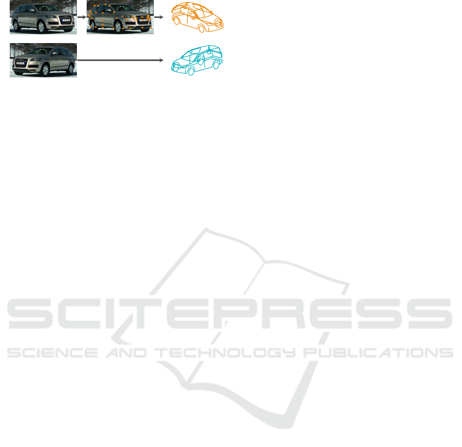
Figure 1: A brief interpretation of the proposed method. We
predict the object 3D shape directly from an input image
(bottom row), instead of fitting a model to the 2D observa-
tions (top row).
detected accurately). The optimization objectives are
usually non-convex and highly non-linear, where the
solutions rely much on the quality of initializations.
The solution can easily get stuck at local minimums.
Compared with the above, the regression-based
method has great merits of utilizing the global geo-
metric constrains. The regressed shape is always con-
strained to reside in the linear subspace constructed
by all training shapes. Motivated by this, we propose
to regress the 3D shape of the object from a single
2D image (see Fig. 1). Although it seems a natural
extension of 2D regression, however, the estimation
problem in 3D shape are very different. Some land-
marks are essentially invisible due to self-occlusion,
accompanied by some visible ones occluded by other
objects. In addition, the appearance of the object is
always more textural than the face, and may change
greatly under various viewpoints. The local landmark
description can cause false alarms in image space due
to the deceptive similarity in feature space (Vondrick
et al., 2013). To address the above drawbacks, we
propose to jointly regress the pose and the 3D shape
of object, and localize the 2D landmarks. The results
of our method benefit from the following highlights
1. Both the appearance and the 2D position infor-
mation are considered for 3D estimation, which
help cope with the discrimination from the local
description of 2D landmarks. The projection po-
sition constrains can prevent the real 3D geomet-
ric shape from severe deformations and encourage
2D landmarks localization.
2. We introduce a method to establish a pairwise an-
notation dataset of the 3D car shape and corre-
sponding 2D landmarks. We use 2D aligned shape
samples and predefined 3D basis to get the 3D
ground-truth.
3. We extend the supervised descent method to im-
plicitly encode the 3D geometric topology into a
series of cascaded regressors.
The remainder of this paper is structured as follows.
In Section 2, we first review some related works. Sec-
tion 3 describes the regression-based model for joint
3D shape estimation and landmarks localization in de-
tail. In Section 5 we do some experiments to validate
the effectiveness of the proposed framework. The last
section draws a conclusion and introduces some fu-
ture works.
2 RELATED WORK
Our work is related to the following research in the
literature, including face alignment, 3D model fitting
of object. Many different types of geometric models
have been applied to machine vision scene. We briefly
review some works on fitting 3D shape model to 2D
image and regression-based alignment methods.
Existing works about multi-view shape estima-
tion can be roughly categorized into two class:
hypothesis-test-based and optimization-based. The
hypothesis-test-based approach (Leotta and Mundy,
2011; Li et al., 2011; Zhang et al., 2012; Zia et al.,
2013b) first generates some hypotheses, and then
finds the correspondences between the hypothesised
and actual images primitives. The hypotheses are
evaluated to find the best that minimizing the shape
predicted errors. Leotta et al. (Leotta and Mundy,
2011) align a kind of deformable model to image by
predicting and matching image intensity. Li et al.
(Li et al., 2011) develop a Bayesian inference algo-
rithm for generating shape and pose hypothesis from
a randomly sampled subsets of landmarks in a first
stage. Then they adopt RANSAC paradigm to iden-
tify the optimal one with robust measure. The shape
and the pose are adjusted by minimizing errors be-
tween the hypothesized and the detected edges in im-
age. Zhang et al.(Zhang et al., 2012) propose to use
gradient-based fitness score to evaluate the match-
ing quality under a generated hypothesis. The object
shape and the pose are recovered through a sampling-
based method, where the samples with better score
are selected as seed for the next generation. In Zia’s
work(Zia et al., 2013b), the local part detectors are
first trained from rendered CAD model across multi-
view images. Then the 3D ASM is fitted to the im-
age by measure similarities with likelihood map un-
der unknown pose. This kind of method suffers from
great time-consuming, amount of occlusions, or lim-
ited applicable under specific discrete viewpoint. In
this paper, we try to establish a 3D shape prediction
framework with low computation complexity.
In optimized-based method, the correspondence
are predefined according to the geometric model, and
the estimation problem became a optimization prob-
lem to find the best fitting parameters. In (Hejrati
and Ramanan, 2012), a part-based model estimate
Joint Monocular 3D Car Shape Estimation and Landmark Localization via Cascaded Regression
223

the 2D positions of landmarks, which are then re-
fined in a second stage by fitting a coarse 3D model
to these landmarks with SfM. The reconstruction of
3D human poses (non-rigid) or 3D car shape (rigid)
given single images has been investigated (Ramakr-
ishna et al., 2012; Lin et al., 2014; Wang et al., 2014;
Zhou et al., 2015; Miao et al., 2016). Ramakrishna
et al.(Ramakrishna et al., 2012) represent the 3D pose
by a linear combination of a series of pose basis that
are learned from motion databases. The pose are pre-
dicted by minimizing the projection residuals of sum
of squared limb lengths as constraint. Towards im-
provement of this work, Wang et al. (Wang et al.,
2014) extend this model by enforce the proportions
of eight selected limbs to be constant, and use `
1
mea-
surement to enhance the robustness. However, these
constraints are not general for all cases while the the
human poses have great variations. In Zhou’s work
(Zhou et al., 2015), they propose a convex relaxation
version of (Ramakrishna et al., 2012) to estimate the
rotation matrix, which need not care the initializa-
tions. Miao et al. (Miao et al., 2016) propose a fast
and robust method to estimate the 3D car shape with
additional type information for initialization. Differ-
ent from these works, (Lin et al., 2014) propose to use
the object class to refine the estimation of the shape,
and the pose parameters are estimated with a modified
version from (Leotta and Mundy, 2011) by evaluate a
Jacobian system. However, in those approaches, pre-
detection of parts or positions of landmarks should be
provided in advance. We aim to develop a method to
predict the 3D shape from images directly.
Most related works to our method are regression-
based method. Boosted regression method (Cristi-
nacce and Cootes, 2007) has been presented early by
Tim Cootes for ASM. Then, there has been numer-
ous papers on face alignment proposed using such a
kind of framework (Saragih, 2011; Xiong and De la
Torre, 2013; Cao et al., 2014; Kazemi and Sullivan,
2014; Tulyakov and Sebe, 2015). Doll
´
ar (Doll
´
ar et al.,
2010) minimizes model parameter errors in the train-
ing, to cascadedly estimated the parametrized varia-
tion of the objects appearance. Instead of regress-
ing each local part independently as (Cristinacce and
Cootes, 2007), Cao et al. (Cao et al., 2014) pro-
pose to learn a vectorial regression function to infer
the whole facial shape from the image and explicitly
minimize the alignment errors over the training data
to exploit the correlations of the landmarks. Although
this method is very accurate, the predicted shapes are
limited as the linear subspace of the training data,
which is not very robust for multiview problems. In
our work, the accuracy of the localization is not the
first important target. Tulyakov et al. (Tulyakov and
Sebe, 2015) have similar motivation with ours. They
succeed the work from (Kazemi and Sullivan, 2014)
by extending the shape invariant splits to 3D space,
and can estimate the face pose accurately. Their work
relies on RGBD dataset, and the 3D regression is only
available under limited view pose changing. In con-
trast, in our method, the training stage and datasets are
all different, and we aim to regress the full 3D shape
of objects.
3 METHOD
In this section, we describe in detail how to regress
the 3D shape from a single viewpoint image with lo-
calizing the 2D landmarks at the same time. We start
from the 3D representation of the shape, and derive
the regression-based shape prediction method. Then
we extend it to the joint estimation of the 3D shape
and the 2D landmarks. In the test stage, an monoc-
ular image and an initial pose of the object are given
as input, and the shape increment is predicted at each
regressor.
3.1 3D Representations
Point Distributed Model (PDM) is widely used for
shape representations such as in face alignment.
By using of such a model, the 3D shape of an
object is represented by n-landmarks PDM X =
[x
1
,y
1
,z
1
,... ,x
n
,y
n
,z
n
]
T
. Suppose the shape X is un-
der the rigid transform of the canonical shape S by
X = Γ(S) = RS + t, (1)
where parameters {R, t}
1
denote 3D rotation and
translation respectively, which specifying the pose of
the object. The canonical shape is learned from a se-
ries of labelled training samples and defined as
S = Bα + µ, (2)
where µ is the mean shape, and B = [B
1
,B
2
,..., B
N
] ∈
R
3n×N
is a group of shape bases . With the above
model, In the above definition, the canonical shape
are denoted in model coordinate system (MCS) and
the 3D shape is defined in world coordinate sys-
tem (WCS). We can get the 2D locations u =
[u
1
,v
1
,. .. ,u
n
,v
n
]
T
with the specific orthogonal pro-
jection matrix
u = sM X, (3)
1
Specifically, 3D rotation R = I
n×n
⊗ R
3×3
and translation
t = I
n×n
⊗ (t
x
,t
y
,t
z
)
T
, where I is identity matrix and ⊗
denotes Kronecker product. Similarly, the camera matrix
in (3) M = I
n×n
⊗ M
2×3
.
ICPRAM 2018 - 7th International Conference on Pattern Recognition Applications and Methods
224

where M is a weak-projection camera matrix (Hart-
ley and Zisserman, 2003) and s is the scaling parame-
ter. Therefore, the objective of 3D shape estimation is
equivalent to estimate the pose parameters and shape
coefficients p = {s, R,t, α} from a given input image.
3.2 Cascaded Regression of 3D Shape
Many cascaded methods can be utilized, such as cas-
caded pose regressor (Eld
´
en and Park, 1999), which
produces object pose as output, and supervised de-
scent method (SDM) (Xiong and De la Torre, 2013),
which aims to output the estimated coordinates. We
start from a general regression-based method which
produce an estimation
b
p of the truth 3D shape param-
eter p of an object from an input image I ∈ R
W ×H
.
b
p can be progressively refined by shape increment
∆p
t
at each stage t (t = 1,. . . , T ) through a cascaded
framework. Then the 3D shape estimation problem
can be described as follows:
∆p
t
= R
t
h(I,g(
b
p
t−1
)), (4)
b
p
t
=
b
p
t−1
+ ∆p
t
, (5)
where u = g(
b
p) generates the 3D shape and projects
them to 2D plane following (1)–(3). h is a non-linear
feature extractor, and φ = h(I,u) ∈ R
Dn×1
in the case
of a D-dimensional feature representation for each
landmark. The features depend on both the image and
the previous estimation, which means that we must
extract the feature at each level in the cascaded frame-
work. R
t
is a regression function learned at t-th stage
and T is the total number of the cascaded regressors.
Encouraged by the success of those methods on
2D face alignment, we design a 3D regression frame-
work for pose estimation by means of SDM. Specif-
ically, we first derive update rule of the 3D shape es-
timation. We find the parameters by fitting the 3D
shape to 2D images through minimizing the differ-
ences between the features extracted against the pro-
jected and the ground-truth landmarks.
b
p = arg min
p
f (p)
= argmin
p
1
2
k
h(I,g(p)) − h (I, g(p
∗
))
k
2
2
Given an initial p
t
at stage t, the cost function can
be approximated by the Taylor expansion and we can
evaluate an incremental parameter ∆p
f (p) = f (p
t
+∆p) =
1
2
k
h(I, g(p
t
+ ∆p)) − φ
∗
k
2
2
(6)
≈ f (p
t
) + J
T
f
∆p +
1
2
∆p
T
H
f
∆p (7)
where φ
∗
denotes the feature at correct landmarks
(manually labelled), and the the Jacobian matrix J
f
and Hessian H
f
are both with respect to f evaluated
on the current parameter p
t
. Take derivation of both
side in (6) with respect to ∆p, and set it to zero, we
can acquire
∆p = −2H
−1
f
J
T
hg
(φ
t
− φ
∗
). (8)
In fact, due to the high non-linearity and non-
differentiable of the feature extractor, we cannot get
the explicit form of Hessian H and Jacobian to min-
imizing (6) . Moreover, it costs expensive numeri-
cal approximations to compute the Hessian. The core
idea behind the SDM is to directly learn the descent
directions from the training data by linear regression,
∆p
t
= −H
−1
f
J
T
hg
φ
t
+ H
−1
f
J
T
hg
φ
∗
= W
t
φ
t
+ b
t
,
where b
t
is a bias estimation based on the fact that in
a testing stage, the ground-truth is unknown. With a
learned regressor, the new estimation is acquired by
following the update rule in (5)
b
p
t
=
b
p
t−1
+ W
t
φ
t−1
+ b
t
. (9)
After a series of regressors, the estimated shape will
be converged to the correct p
∗
for each corresponding
images in training set.
In previous works on multi-view face alignment,
each landmark is represented in 2D coordinates, or
extended by adding a binary label to each point to
indicate the visibility, or use the 3D coordinates di-
rectly. In our model, we have some differences from
those approaches. In each stage, we parametrize the
under-estimated shape and pose, which can normal-
ize the effect from various pose in the training sam-
ples. What’s more, both the object appearance and 2D
geometric consistence are considered in the proposed
model. In the next, we will introduce the model in
detail.
3.3 Joint Estimation with 2D Alignment
We add a 2D alignment item to enforce the match-
ing of the 2D landmarks under the model projec-
tion with parameter p with the ground-truth 2D land-
marks. This can help to avoid the possible ambiguity
when use the local image patch to describe each land-
mark, due to the fact of the lack of global constraints.
The objective function became
b
p = arg min
p
f (p)
= argmin
p
1
2
h
k
h(I,g(p)) − h (I, g(p
∗
))
k
2
2
+ β
k
g(p) − g(p
∗
)
k
2
2
i
,
Joint Monocular 3D Car Shape Estimation and Landmark Localization via Cascaded Regression
225

which means that, the projected shape and the cor-
responding appearance should be consistent with the
ground-truth. Therefore, given an initial p
t
at stage
t, the cost function can be approximated by the Tay-
lor expansion, and we can evaluated an incremental
parameter ∆p
f (p) = f (p
t
+ ∆p) =
1
2
h
k
h(I, g(p
t
+ ∆p)) − φ
∗
k
2
2
+ β
k
g(p
t
+ ∆p) − u
∗
k
2
i
≈ f (p
t
) + J
f
(p
t
)∆p +
1
2
∆p
T
H
f
∆p (10)
Take derivation of both side in (10) with respect to
∆p, and set it to zero, we can acquire
∆p = −H
−1
f
[(J
h
J
g
)
T
(φ
t
− φ
∗
) + βJ
T
g
(u
t
− u
∗
)]
= −H
−1
f
(J
h
J
g
)
T
φ
t
− βH
−1
f
J
T
g
u
t
+ H
−1
f
(J
h
J
g
)
T
φ
∗
+ βH
−1
f
J
T
g
u
∗
= Wφ
t
+ βGu
t
+ b. (11)
Therefore, we can get a new update rule as the follow-
ing equation
b
p
t
=
b
p
t−1
+ W
t
φ
t−1
+ βG
t
u
t−1
+ b
t
. (12)
where the regressor is R
t
= {W
t
,G
t
,b
t
}.
3.4 Learning and Test
In this section, we describe in detail how to
learn the regressor sequences {R
1
,R
2
,. .. ,R
T
} from
the training sets. Given some images I =
{I
1
,I
2
,. .. ,I
M
} with the labelled pose and shape pa-
rameters {p
1
∗
,p
2
∗
,. .. ,p
M
∗
} as training-set, each regres-
sor R
t
= {W
t
,G
t
,b
t
} can be learned by
min
W
t
,G
t
,b
t
M
∑
i=1


p
i
∗
−
b
p
i
t−1
− W
t
φ
i
t−1
− βG
t
b
u
i
t−1
− b
t


2
2
,
(13)
where ∆p
∗
t
= p
∗
−
b
p
t−1
is the objective update. Since
we extract HoG features in a neighbour region for
each landmark, the dimension number will be very
large. This leads to over-fitting easily of the learned
regressors, and high computation. To avoid this prob-
lem, we consider to imposing a penalty item to regu-
larize object function in (3.4). And the parameter λ
t
is
selected to control the strength of the penalty. There-
fore, the objective function for learning t-th regressor
is reformulated as follows
min
W
t
,G
t
,b
t
M
∑
i


∆p
∗i
t
− W
t
φ
i
t−1
− βG
t
b
u
i
t−1
− b
t


2
2
+ λ
t

kW
t
k
2
F
+
k
G
t
k
2
2
+ kb
t
k
2
2

, (14)
where we find that β = 0.1 is appropriate. It is easily
solved in closed-form. However, training stage needs
a lot of perturbation samples to enhance the general-
ity of the model, where many outliers are inevitable.
Therefore, solve (14) can result in great estimation
bias. In real applications, we use support vector re-
gression with ε-loss (Ho and Lin, 2012) instead of
quadratic loss to penalize large error samples, which
can strengthen robustness to outliers. The equivalent
dual problem can also be solve with low computation
cost.
Algorithm 1: Training Regressor Sequences.
Input: K training images {I
i
}
K
i=1
with manually la-
belled shape ground-truth p
i
∗
= {s
i
∗
,R
i
∗
,α
i
∗
}
Output: T regressors: {W
t
,G
t
,b
t
}
T
t=1
1: Initialize Generate M training perturbation pa-
rameters
2: for t ← 1 to T do
3: for i ← 1 to M do
4: ∆p
∗,i
t
← p
i
∗
− p
i
t−1
// The objective update
5: u
i
t−1
← s
i
t−1
M R
i
t−1
(Bα
i
t−1
+µ)+t
t−1
// Pro-
jection to 2D according to shape and pose
6: φ
i
t−1
= h(I
i
,u
i
t−1
) // Extract HOG features
7: end for
8: R
t
= {W
t
,G
t
,b
t
} is learned by solving (14)
9: for all i do
10: p
i
t
← p
i
t−1
+ W
t
φ
i
t−1
+ G
t
u
i
t−1
+ b
t
11: end for
12: end for
The supervised learning of the model needs pre-
generated perturbation parameters according to cer-
tain distribution. In the training stage, we first get
the 2D mean shape from the labelled data. Then, we
generate randomly some shifts of the mean shape uni-
formly as the perturbations and calculate the pose and
3D shape parameters. Hence the objective updates are
acquired by calculate the parameter differences be-
tween the shifted and labelled shapes. The full train-
ing procedure of the proposed training method is sum-
marized in Algorithm 1.
To apply the model to a new input, we first give
a initial pose and shape parameters, then extract fea-
tures. To get a reliable pose guess effectively, we first
get a coarse object detection result, which is helpful
to shrink the search range to improve the landmark
localization. Here we utilize Deformable Part-based
Model (DPM) (Felzenszwalb et al., 2010) to get a
bounding-box, which has shown the-state-of-the-art
performance for object detection.
The initial shape parameters should be generated
by the procedure as the same as the training step, so
as to ensure the same distribution, which is important
ICPRAM 2018 - 7th International Conference on Pattern Recognition Applications and Methods
226

Algorithm 2: 3D Shape Inference.
Input: A test image J, and the learned regressors
{W
k
,G
k
,b
k
}
T
k=1
Output: u
o
,p
1: Initialization the shape parameters p
0
=
{s
0
,R
0
,t
0
,α
0
}
2: for k ← 1 to T do
3: u
k−1
← s
k−1
M R
k−1
(Bα
k−1
+ µ) + t
k−1
4: φ
k−1
= h(J, u
k−1
)
5: p
k
← p
k−1
+ W
k
φ
k−1
+ G
k
u
k−1
+ b
k
6: end for
7: u
o
← s
T
M R
T
(Bα
T
+ µ) + t
T
8: p ← {s
T
,R
T
,t
T
,α
T
}
to guarantee the convergence of updating. Using the
trained regressors cascadedly, the inferred parameters
are used to calculate the shape as described in Algo-
rithm 2.
4 DATA ANNOTATION
To train such a kind of framework, one should per-
form annotation of the training samples. For 3D
cases, it is not enough to train the model with just
2D locations of the object shape. Moreover, it is also
difficult to label the third dimension of the landmarks
by only observing a single monocular image. And
there are rarely datasets provide the corresponding 3D
annotations to the 2D. To the best of our knowledge,
there are no images and shapes pairwise annotated car
dataset. Here, we use the available 3D shape data pro-
vided by (Zia et al., 2013a) to annotate. As showed
in Fig. 2, each 3D model contains 36 salient points,
which are selected from CAD data to cover important
features for description of the object.
-0.5
0
3
0.5
1
2
1
0
-1
1
-2
0
-1
-3
Figure 2: The training 3D
shapes are plotted together,
where their scales are nor-
malized in a fixed-size box.
Figure 3: The training im-
ages under specified train-
ing view with the 2D anno-
tated landmarks showed.
We first calculate the pose parameters and shape
representations from the manually defined 2D land-
marks. Given some 2D images annotated with 2D the
landmarks x, and the predefined or pre-learned shape
bases B, we first estimate the camera pose parameters
and the shape representations by the following opti-
mization problem.
arg min
s,R,t,α
1
2





x − sM R
N
∑
i=1
B
i
α
i
+ µ
!
+ t





2
F
+ η
k
α
k
2
2
s.t. R
T
R = I
(15)
Many approaches have been proposed such as in (Ra-
makrishna et al., 2012; Zhou et al., 2015; Miao et al.,
2016) to solve similar problems with different formu-
lations. To solve the problem (4), a common approach
is alternatively optimizing the camera pose and the
shape representations. This kind of method highly re-
lies on the initializations, while bad ones can gener-
ate infeasible 3D shapes. The 3D annotation from 2D
should recovery the real geometric structure. There-
fore, we adopt the convex relaxation method (Zhou
et al., 2015) to make the 3D annotations. The re-
projected points in 2D are regarded as the new 2D
annotations. The regularization parameter η is set to
0.1, in avoid of large errors between re-projected and
the original labelled points.
Another issue is about how to represent the three
dimensional rotation matrix R. It is not appropriate
to directly optimize the 9-dimensional space matrix,
which may lose the manifold constraints. Here we
use a Rodrigues’ vector w = [w
x
,w
y
,w
z
]
T
, which is
an axis-angle representation of rotation. Then the axis
of rotation is equal to the direction of w, and the an-
gle of rotation against this axis is equal to the magni-
tude θ =
k
w
k
. According to a Lie-algebraic deriva-
tion (Marsden and Ratiu, 1999), the exponential map
has a closed-form expression to transform a rotation
vector w into a 3 × 3 rotation matrix R by
R(w) = e
[w]
×
= I
3×3
+
[w]
×
θ
sinθ +
[w]
2
×
θ
2
(1 − cosθ)
(16)
where [w]
×
is the skew-symmetric cross-product ma-
trix of w.
[w]
×
=


0 −w
z
w
y
w
z
0 −w
x
−w
y
w
x
0


To retrieve the Rodrigues’ vector from the rotation
matrix, we first calculate the trace of R to get the angle
θ
θ = 2 cos
−1
p
tr(R) + 1
2
,
and the axis of rotation w is recovered as
w =
θv
k
v
k
, v =


R(3,2) − R(2, 3)
R(1,3) − R(3, 1)
R(2,1) − R(1, 2)


. (17)
We then artificially simulate a large amount of data
from K annotations. we generate M random perturba-
tions as training data, according to the same procedure
described in 3.4.
Joint Monocular 3D Car Shape Estimation and Landmark Localization via Cascaded Regression
227

5 EXPERIMENTS
To show the performance to the proposed framework,
we assess the accuracy of pose and shape estimation
in terms of both viewpoints and empirical error distri-
bution. We present the landmarks localization results
on different views images and different types of cars,
both the 2D results and the 3D fitted results. We also
give the visual results of the shape reconstruction on
the test dataset.
5.1 Dataset
Training Data: We use the annotated data from
(Zia et al., 2013b). The image data has been
roughly divided into 8 discretized views as the
Front, Front-Left, Left, Rear-Left, Rear, Rear-Right,
Right, and Front-Right of the car.The left side view
pose is set as 0
◦
. The 2D cars are annotated by
8,22, 18,22, 8,22, 18,22 landmarks for each view-
point respectively. The cars in this dataset span a wide
variety of type, size under different illumination con-
ditions and background environment with various par-
tial occlusions. There are totally 2910 images across
all the whole dataset. We randomly choose 70 per-
centage of them for training, and use the rest images
to test in each viewpoint. For the purpose of train-
ing on a consensus feature scale, and control the pose
variety, the labelled 2D landmarks in all the training
images are approximately aligned to a reference tem-
plate as a normalized input. Fig. 3 shows some train-
ing instances under different viewpoints.
3D model Data: As introduced in section 4, the 3D
point-based models are trained on a set of labelled
3D CAD models. It provides a deformable wireframe
representation based on a set of vertices of the object
class of interest. We used the car model trained by the
author (Zia et al., 2013a). Each shape is represented
by a 36-landmarks point distribution model. In our
experiments, we use 30 different samples as the shape
basis. They are rich enough to cover the basic types
of cars.
5.2 Experimental Settings
Feature: To train the regression models, we should
generate the local patches to be used for feature ex-
traction. For each landmark, we extract an image
patch with 40 × 40 pixels size to capture the local
appearance. Considering the excellent performances
of HoG descriptor in detection (Saragih et al., 2011;
Andriluka et al., 2009; Saragih, 2011), we then com-
puted HoG features (Dalal and Triggs, 2005) on each
extracted patch to describe the local appearance. We
set the block size to 2 × 2 cells, where the cell size is
8 × 8 pixels. We compute HoG descriptors on over-
lapping grids of spatial blocks densely, with gradients
extracted on 9 orientations. The HoG dimension for
each local patch is 4 × 4 × 2 × 2 × 9 = 576. This lead
to extremely high-dimensional feature vectors after
concatenation, thus we use principle component anal-
ysis to reduce the dimension and whiten the features.
With 96% energy preserved, the corresponding eigen-
vectors are selected as the feature whitening parame-
ters.
Model:. There are some parameters about the model
to be set-up. The regularization parameter λ in (14) is
selected by cross-validation, and finally fixed to 0.1 in
each training stage. To determine how many cascaded
stages should be used, we record the objective update
values ∆p
∗
in the training process. Fig. 4 presents the
∆p
∗
changing with respect to the training stage. We
set the total stage as T = 5 based on the fact that ∆p
∗
changes very slowly with a very small deviation from
stage 4 to 5. To efficiently solve the objective in (14)
1 2 3 4 5
Stage
0
0.5
1
1.5
2
2.5
k∆p
∗
k
Figure 4: The objective update changes with training stage.
as mentioned above, we use the LibSVM (Chang and
Lin, 2011), where the tolerance threshold is fixed to
10
−6
.
Evaluation: To evaluate the accuracy of the pose esti-
mation, we use different metric to measure the errors.
The scale estimation accuracy are computed by
d
s
(ˆs,s
g
) =




ˆs
s
g
− 1




,
which measure the disagree extent to the ground-
truth. As for the 3D rotation, we follow a loga-
rithm map definition in (Engø, 2001) to calculate the
geodesic distance of two rotation matrix in SO(3). It
is defined as
d
R
(
b
R,R
g
) =



log

b
R
T
R
g




F
.
For the translation and re-project 2D points errors,
we use the root-mean-square-error (RMSE) as the
evaluation criterion. The in-pixel localization errors
are then normalized by the bounding-box size of the
ground-truth shape, which is computed as the mean
ICPRAM 2018 - 7th International Conference on Pattern Recognition Applications and Methods
228

0 0.5 1 1.5 2
Scale Error
0
0.5
1
Ratio
Ours
SDM-3D
SDM2D+Manopt
SDM2D+ALT
0 1 2 3
Rotation Error
0
0.5
1
Ratio
Ours
SDM-3D
SDM2D+Manopt
SDM2D+ALT
0 1 2 3
Translation Error
0
0.5
1
Ratio
Ours
SDM-3D
SDM2D+Manopt
SDM2D+ALT
1 2 3 4 5 6 7 8
Viewpoint
0
0.1
0.2
Mean Error
Ours
SDM-3D
SDM2D+Manopt
SDM2D+ALT
1 2 3 4 5 6 7 8
Viewpoint
0
0.5
1
Mean Error
Ours
SDM-3D
SDM2D+Manopt
SDM2D+ALT
1 2 3 4 5 6 7 8
Viewpoint
0
0.5
1
1.5
Mean Error
Ours
SDM-3D
SDM2D+Manopt
SDM2D+ALT
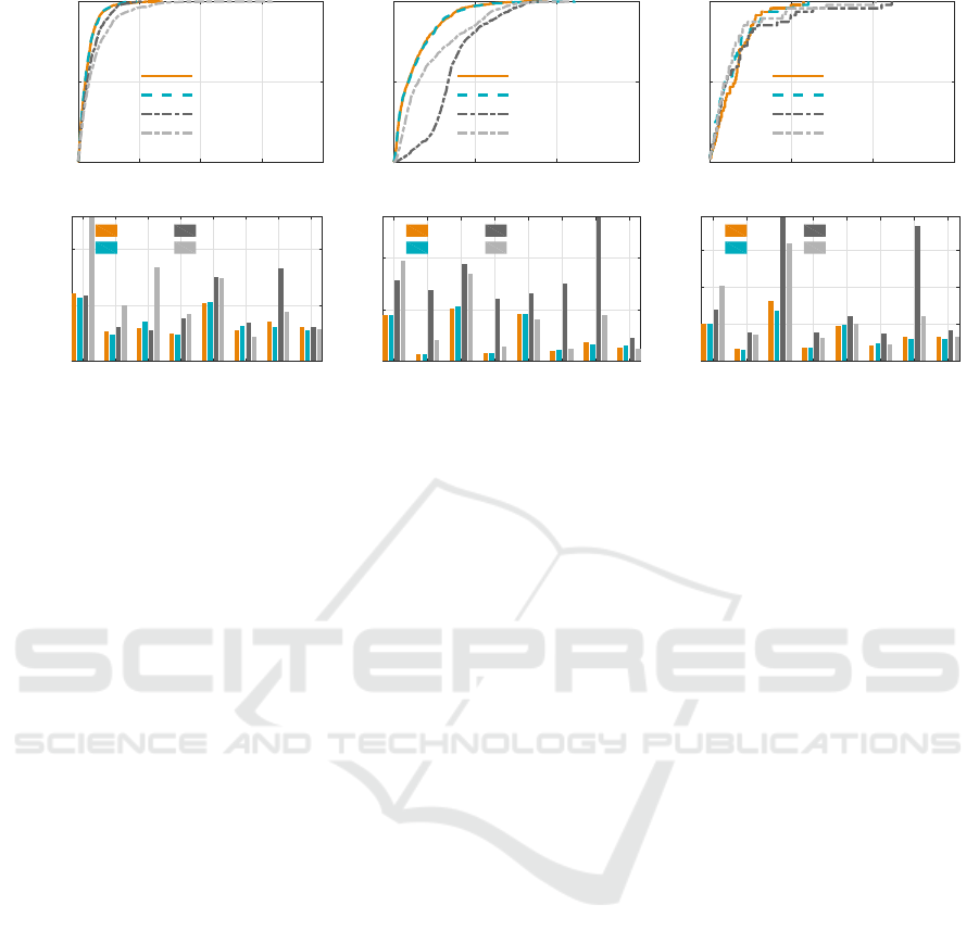
Figure 5: Cumulative error distribution of the pose estimation (top row) and the mean accuracy with respect to the viewpoints
(bottom row). From the left to the right are the results on the scale s, rotation R and translation t. Ratio means that the
proportion of the test images.
of the width and height. Then we investigate the 3D
shape recovery performance under the second layer
and the refined localization results. We use the Pro-
crustes distance errors (PDE) (Dryden and Mardia,
1998) to measure the accuracy for the estimated 3D
shape. The Procrustes distance errors are computed
between the predicted 3D shape
b
X and the ground-
truth 3D annotation X
g
. Specifically, the Procrustes
distance between
b
X and X
g
is
d
X
(
b
X,X
g
) = inf
Γ
T
Γ=I
3
,β>0



b
X − βΓX
g



F
,
where I
3
denotes identity matrix. This measurement
can avoid from the influences from the inaccurate
pose estimation while we only focus the 3D shape it-
self.
Comparison: We compare the proposed method with
the two kinds of approaches. One is the 3D regres-
sion method derived in Section 3.2, which is an ex-
tent version of the SDM framework to 3D shape es-
timation. The other kind of method is a two-step es-
timation framework. In the first step, 2D landmarks
are firstly localized by certain approaches. In the sec-
ond step, the 3D shape is reconstructed by solving the
same problem in annotation procedure (4), provided
the results in step one. In comparison, we realize
the 2D regression by SDM to detect the landmarks as
the results in the first step. Then, we use a modified
the method proposed in (Ramakrishna et al., 2012) to
solve (4). We also compare a different rotation esti-
mation algorithm by manifold optimization (Boumal
et al., 2014).
5.3 Quantitative Results
We access the estimation performance of the pose and
3D shape, and use the re-projected points to evaluate
the localization accuracy.
5.3.1 Comparison of Pose Estimation
First, We present the pose estimation results in Fig. 5.
According to the cumulative scale error distribution,
the proposed method has similar performance with
SDM-3D. The percentage with errors no large than
0.5 is 99.66 and improve 3.44% and 19.98% com-
pared with the two two-step framework. As for the
rotation estimation, the accuracy by SDM-3D is as
well as the joint framework, while the results by the
other two methods are far away from the proposed
method. The translation error distribution demon-
strates that the proposed method is not the best when
the normalised error is within 0.5. However, we no-
tice that the proposed method have significantly ad-
vantages in rotation estimation. The reason can be
that, the rotation in the two-step framework is solved
as non-convex constraint, and its numerical precision
can not be guaranteed.
For the results under different viewpoints, all these
methods have better performance on view 2, 4, 6, 8
than the left viewpoints for the pose estimation. This
can be interpreted from the number of visible land-
marks which are used for 3D reconstruction. The ob-
servations under front-left, front-right, rear-left and
rear-right can provide more information to estimate
the 3D car shape than the other viewpoints. The pro-
posed method is not better than the compared ones on
Joint Monocular 3D Car Shape Estimation and Landmark Localization via Cascaded Regression
229

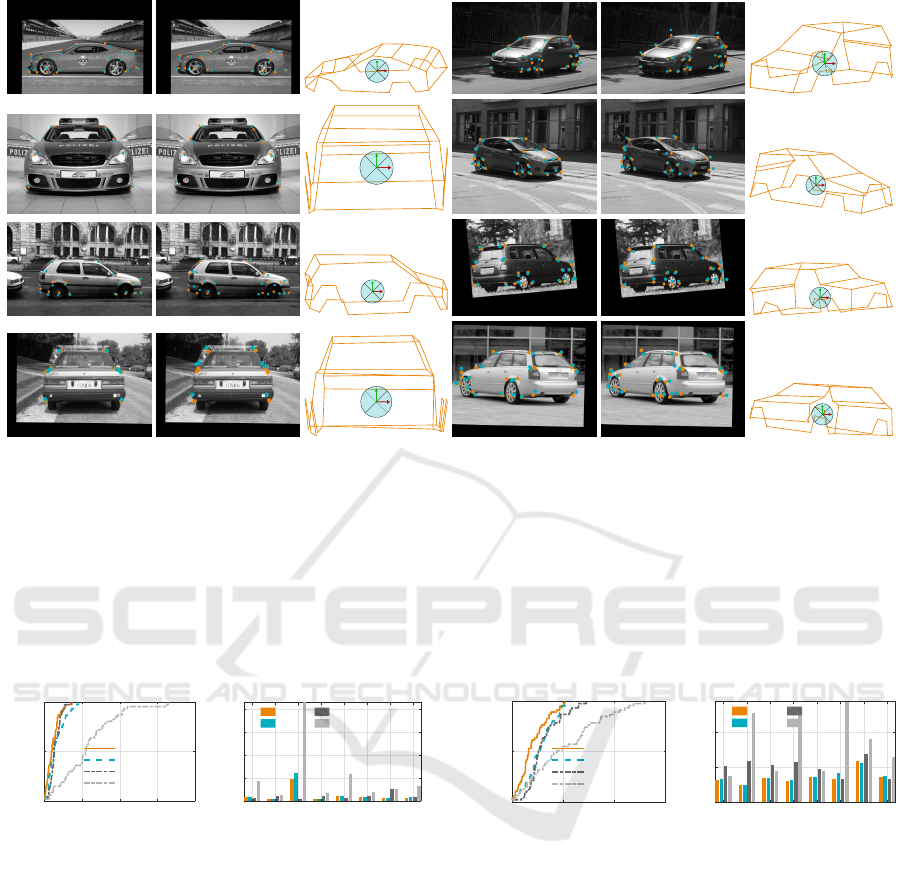
Figure 6: The qualitative localization results and the visual results of the 3D shape estimation. From left to right in each
triple-group, we present the 2D landmarks localization results by (Xiong and De la Torre, 2013) and the proposed method,
and the predicted 3D shape by our method respectively. The origin circles show the ground-truth and the blue ones denote the
re-project results.
average, where the performance degeneration may be
caused by the joint estimation (e.g. the translation er-
rors under front or rear samples are larger than SDM-
3D). We also find that, the rotation estimation cannot
be guaranteed by Manopt toolbox for some specific
viewpoints.
0 0.1 0.2 0.3 0.4
RMSE
0
0.5
1
Ratio
Ours
SDM-3D
SDM2D+Manopt
SDM2D+ALT
1 2 3 4 5 6 7 8
Viewpoint
0
0.2
0.4
0.6
0.8
Mean Error
Ours
SDM-3D
SDM2D+Manopt
SDM2D+ALT
Figure 7: Cumulative distribution of localization errors on
the test-set. The re-projection error is used to measure the
landmarks localization accuracy.
5.3.2 Comparison of Shape Estimation
Then, we evaluate the shape estimation by assess the
accuracy of 2D landmarks localization and 3D shape
reconstruction. We use the re-projected landmarks of
the estimated 3D shape as the 2D localization results.
In other words, this measure reflects how well the
estimations matching with the observations. Fig. 7
presents the error distribution of different compared
methods. The proposed method shows better perfor-
mance, which benefits from the more accurate esti-
mation of the pose and the 3D shape. In perspective
of different viewpoints, our method achieve lower er-
rors compared with the other three except for the rear
view. The SDM2D+Manopt have also good match-
ing results, although the rotation matrix is not es-
timated perfectly. This phenomenon demonstrates
that, SDM2D+Manopt tends to make the 2D match-
ing more accurate rather than 3D shape estimation un-
der the same parameters setup for problem (4).
0 0.2 0.4 0.6
3D Error
0
0.5
1
Ratio
Ours
SDM-3D
SDM2D+Manopt
SDM2D+ALT
1 2 3 4 5 6 7 8
Viewpoint
0
0.2
0.4
Mean Error
Ours
SDM-3D
SDM2D+Manopt
SDM2D+ALT
Figure 8: The 3D estimation results.
Finally, we examine the 3D prediction accuracy
on this multiview car test-set. Fig. 8 shows the 3D
shape estimation results. Compared with the two-
step framework, the proportion of samples with nor-
malised errors within 0.15 are 46.81% and 65.96%
higher than SDM2D+Manopt and SDM2D+ALT re-
spectively. The performance has been improved
8.51% to SDM3D. The reason can be that, our
method enhance the landmarks position constraints
to provide more information for 3D shape estimation.
What’s more, we find that bad results are acquired by
SDM2D+ALT method. This means alternative opti-
mization is sensitive to the initialization of the solu-
tion. In contrast, the two-step framework by Manopt
is more robust.
ICPRAM 2018 - 7th International Conference on Pattern Recognition Applications and Methods
230

5.4 Qualitative Results
To show the shape estimation results intuitively, we
present the visual results of landmarks localization
and the 3D car shape with the estimated camera pose
in Fig. 6. The results cover various cases with differ-
ent viewpoints and type of the car. It can be obviously
observed that, the localization results by the proposed
method appear nearly the same to the results of di-
rectly 2D regression method (SDM2D). At the same
time, the 3D shape and camera pose can be seen well
estimated.
6 CONCLUSIONS
In this paper, we have proposed a method for 3D
shape reconstruction and landmarks localization. By
representing the 3D shape as a linear combination of
a set of shape bases, we have proposed a cascaded
framework to regress the global geometry structure
and the object pose. We proposed a new objective
to train the regressors, by minimizing the appearance
and the shape differences at the same time, which can
overcome the ambiguity of the landmarks description
in feature space. Experimental results showed com-
petitive performance on shape and pose estimation
without degenerating the localization performance,
compared with some previous methods.
ACKNOWLEDGEMENTS
This work was supported in part by the National
Basic Research Project of China (973) under Grant
2013CB329006 and in part by National Natural Sci-
ence Foundation of China under Grant 61622110,
Grant 61471220, Grant 91538107.
REFERENCES
Andriluka, M., Roth, S., and Schiele, B. (2009). Pictorial
structures revisited: People detection and articulated
pose estimation. In Proc. CVPR, pages 1014–1021.
IEEE.
Boumal, N., Mishra, B., Absil, P.-A., and Sepulchre, R.
(2014). Manopt, a matlab toolbox for optimization
on manifolds. J. Mach. Learn. Res., 15:1455–1459.
Cao, X., Wei, Y., Wen, F., and Sun, J. (2014). Face align-
ment by explicit shape regression. Int. J. Comput. Vis.,
107(2):177–190.
Chang, C.-C. and Lin, C.-J. (2011). LIBSVM: A library
for support vector machines. ACM Trans. Intell. Syst.
Technol., 2:27:1–27:27.
Cootes, T. F., Edwards, G. J., and Taylor, C. J. (2001). Ac-
tive appearance models. IEEE Trans. Pattern Anal.
Mach. Intell., 23(6):681–685.
Cristinacce, D. and Cootes, T. F. (2007). Boosted regression
active shape models. In BMVC, volume 1, page 7.
Dalal, N. and Triggs, B. (2005). Histograms of oriented gra-
dients for human detection. In Proc. CVPR, volume 1,
pages 886–893. IEEE.
Doll
´
ar, P., Welinder, P., and Perona, P. (2010). Cascaded
pose regression. In Proc. CVPR, pages 1078–1085.
IEEE.
Dryden, I. and Mardia, K. (1998). Statistical analysis of
shape. John Wiley & Sons.
Eld
´
en, L. and Park, H. (1999). A procrustes problem on the
stiefel manifold. Numer. Math., 82(4):599–619.
Engø, K. (2001). On the bch-formula in so(3). BIT Numer-
ical Mathematics, 41(3):629–632.
Felzenszwalb, P. F., Girshick, R. B., McAllester, D., and
Ramanan, D. (2010). Object detection with discrimi-
natively trained part-based models. IEEE Trans. Pat-
tern Anal. Mach. Intell., 32(9):1627–1645.
Ferrari, C., Lisanti, G., Berretti, S., and Del Bimbo, A.
(2017). A dictionary learning based 3d morphable
shape model. IEEE Trans. Multimedia.
Guo, Y., Sohel, F., Bennamoun, M., Wan, J., and Lu, M.
(2014). An accurate and robust range image registra-
tion algorithm for 3d object modeling. IEEE Trans.
Multimedia, 16(5):1377–1390.
Hartley, R. and Zisserman, A. (2003). Multiple view geom-
etry in computer vision. Cambridge university press.
Hejrati, M. and Ramanan, D. (2012). Analyzing 3d objects
in cluttered images. In NIPS, pages 593–601.
Ho, C.-H. and Lin, C.-J. (2012). Large-scale linear support
vector regression. J. Mach. Learn. Res., 13(1):3323–
3348.
Kazemi, V. and Sullivan, J. (2014). One millisecond face
alignment with an ensemble of regression trees. In
Proc. CVPR, pages 1867–1874.
Leotta, M. J. and Mundy, J. L. (2011). Vehicle surveillance
with a generic, adaptive, 3d vehicle model. IEEE
Trans. Pattern Anal. Mach. Intell., 33(7):1457–1469.
Li, Y., Gu, L., and Kanade, T. (2011). Robustly aligning
a shape model and its application to car alignment of
unknown pose. IEEE Trans. Pattern Anal. Mach. In-
tell., 33(9):1860–1876.
Lin, Y.-L., Morariu, V. I., Hsu, W., and Davis, L. S.
(2014). Jointly optimizing 3d model fitting and fine-
grained classification. In Proc. ECCV, pages 466–480.
Springer.
Marsden, J. E. and Ratiu, T. (1999). Introduction to me-
chanics and symmetry: a basic exposition of classical
mechanical systems. Springer-Verlag.
Miao, Y., Tao, X., and Lu, J. (2016). Robust monocular 3d
car shape estimation from 2d landmarks. IEEE Trans.
Circuits Syst. Video Technol.
Nair, P. and Cavallaro, A. (2009). 3-d face detection, land-
mark localization, and registration using a point dis-
tribution model. IEEE Trans. Multimedia, 11(4):611–
623.
Joint Monocular 3D Car Shape Estimation and Landmark Localization via Cascaded Regression
231

Ramakrishna, V., Kanade, T., and Sheikh, Y. (2012). Recon-
structing 3d human pose from 2d image landmarks. In
Proc. ECCV, pages 573–586. Springer.
Saragih, J. (2011). Principal regression analysis. In Proc.
CVPR, pages 2881–2888. IEEE.
Saragih, J. M., Lucey, S., and Cohn, J. F. (2011). De-
formable model fitting by regularized landmark mean-
shift. Int. J. Comput. Vis., 91(2):200–215.
Tan, T.-N., Sullivan, G. D., and Baker, K. D. (1998). Model-
based localisation and recognition of road vehicles.
Int. J. Comput. Vis., 27(1):5–25.
Tulyakov, S. and Sebe, N. (2015). Regressing a 3d face
shape from a single image. In Proc. ICCV, pages
3748–3755. IEEE.
Vondrick, C., Khosla, A., Malisiewicz, T., and Torralba, A.
(2013). Hoggles: Visualizing object detection fea-
tures. In Proc. ICCV, pages 1–8.
Wang, C., Wang, Y., Lin, Z., Yuille, A. L., and Gao, W.
(2014). Robust estimation of 3d human poses from
a single image. In Proc. CVPR, pages 2369–2376.
IEEE.
Weng, R., Lu, J., Tan, Y.-P., and Zhou, J. (2016). Learning
cascaded deep auto-encoder networks for face align-
ment. IEEE Trans. Multimedia, 18(10):2066–2078.
Xiang, Y. and Savarese, S. (2012). Estimating the aspect
layout of object categories. In Proc. CVPR, pages
3410–3417. IEEE.
Xiong, X. and De la Torre, F. (2013). Supervised descent
method and its applications to face alignment. In Proc.
CVPR, pages 532–539. IEEE.
Zhang, Z., Tan, T., Huang, K., and Wang, Y. (2012).
Three-dimensional deformable-model-based localiza-
tion and recognition of road vehicles. IEEE Trans.
Image Process., 21(1):1–13.
Zhou, X., Leonardos, S., Hu, X., and Daniilidis, K. (2015).
3d shape reconstruction from 2d landmarks: A convex
formulation. In Proc. CVPR, pages 4447–4455. IEEE.
Zia, M. Z., Stark, M., Schiele, B., and Schindler, K.
(2013a). Detailed 3d representations for object recog-
nition and modeling. IEEE Trans. Pattern Anal. Mach.
Intell., 35(11):2608–2623.
Zia, M. Z., Stark, M., and Schindler, K. (2013b). Ex-
plicit occlusion modeling for 3d object class represen-
tations. In Proc. CVPR, pages 3326–3333. IEEE.
ICPRAM 2018 - 7th International Conference on Pattern Recognition Applications and Methods
232