Plantation Rows Identiﬁcation by Means of Image Tiling and Hough

Transform

Guilherme Afonso Soares, Daniel Duarte Abdala and Mauricio Cunha Escarpinati

Faculty of Computing, Federal University of Uberl

andia, Uberl

andia, Brazil

Keywords:

Image Processing, Crop Lines Identiﬁcation, Precision Agriculture.

Abstract:

In this work we address the problem of plantation rows identiﬁcation on UAV imaged coffee crop ﬁelds. A fair

number of approaches address the problem using the Hough Transform. However it assumes the plantation

lines are straight which is hardly the case in Aerial images. We propose a tiling scheme which allows one to

acceptably approximate the rows inside each tile to straight lines making it feasible to apply the Hough Trans-

form. Experimental results compared to ground truths seems to indicate the proposed approach successfully

approximate real plantation rows.

1 INTRODUCTION

Nowadays precision agriculture is heavily dependent

on imaging and mapping technologies e.g. for esti-

mating growth (Kataoka et al., 2003), or identifying

other important agronomic characteristics (Sankaran

et al., 2015) such as nitrogen stress (Blackmer and

Schepers, 1996). Advances in Unmanned Aerial Ve-

hicles - UAV - technology led to its widespread popu-

larization. With the corresponding drop in operational

costs even smaller plantations are now able to afford

the usage of imaging aided technologies.

The latest economic report by the Association

of Unmanned Aerial Vehicle International (AUVSI,

2013) points out the agricultural market is by far the

largest segment for UAVs. In the United States alone

it is forecast to create thousands of new jobs and con-

siderable revenue and taxes. With the market growth

production costs are expected to drop. It in turn will

allow smaller enterprises such as family and small

agricultural cooperatives (Turner et al., 2016) to bene-

ﬁt from the diminished operational costs to also make

use of precision agriculture aided by UAVs. Other

countries like Japan are also making extensive use of

UAVs in agriculture and in Brazil a number of startup

companies such as Sensormap, Orion and Sensix to

cite just a few are producing and commercializing

UAVs.

There are obvious market for UAVs been agricul-

ture the most prominent example. The technology

is mature and the market offers a number of cost ef-

fective solutions. However, the market lacks reliable

software to process the remote sensed data. With

the dawn of UAVs to adapt solutions derived from

previously used aerial vehicles would be the obvious

choice. However, the available software was devel-

oped for vehicles that capture images on either high

(planes and helicopters) or ultra-high (satellites) alti-

tudes. The problem is further complicated by the fact

that much of the existing software on the market is

proprietary.

In this context the need of developing new soft-

ware able to dealing with low or medium altitude im-

agery became clear. Additionally the development of

new, better and cheaper imaging sensors opens new

avenues of exploration.

New application niches are opening in precision

agriculture aided by low/average altitude remote sens-

ing. Among them, a key problem is to identify where

the planting rows are located in the imaged ﬁeld. This

procedure is important for crop planning, produc-

tion estimation, plant counting, harvesting and early

correction of failures in sowing. Considering the

imaging processing techniques available, the Hough

Transform (Hough, 1962) ﬁgures as an initial clear

choice. As shown in (Illingworth and Kittler, 1988)

it is widely used in identifying ﬁxed parameterized

shapes formed by points on images. The basic Hough

Transform works well for regular geometric forms,

like straight lines and circles, but it can also be used

to ﬁnd arbitrary shapes (Ballard, 1981). However it

requires that the object shape to be known in advance,

which limits its application on plantation row track-

ing. It is worth notice that sometimes crops follow

Soares, G., Abdala, D. and Escarpinati, M.

Plantation Rows Identiﬁcation by Means of Image Tiling and Hough Transform.

DOI: 10.5220/0006657704530459

In Proceedings of the 13th International Joint Conference on Computer Vision, Imaging and Computer Graphics Theory and Applications (VISIGRAPP 2018) - Volume 4: VISAPP, pages

453-459

ISBN: 978-989-758-290-5

453

the terrain, are hindered by obstacles or any other ar-

bitrary unknown geographical feature. Nonetheless a

number of solutions were proposed using the Hough

Transform as basis.

In (Ronghua and Lijun, 2011) a crop row detec-

tion algorithm is presented using as basis the Hough

Transform. It works on ground level images taken

manually with a hand camera. In (Leemans and

Destain, 2006) a row localization method is proposed

in which uses an adaptation of the Hough Transform.

It also works on ground level images captured by a

camera mounted on a tractor. The method is speciﬁ-

cally tunned to deal with early sowing and was tested

only with chicory. In (Søgaard and Olsen, 2003)

approaches the problem from a similar perspective.

Since those methods operate on images captured by

tractor mounted cameras, they make the assumption

that plantation rows can be approximated by straight

lines. In (Garc

ıa-Santill

an et al., 2017) such approxi-

mation is not used. However, it also uses ground level

images. It assumes a few properties about the images,

such as the fact that there will be roughly vertical lines

starting at the image bottom. It also uses a local ap-

proach, whereas this work proposes to ﬁnd the lines

on the whole mapped area. There are approaches for

ﬁnding general curves from a set of points, as de-

scribed in (Lee, 2000). These approaches require the

set of points to comprise only one curve.

Differently from ground level imagery, in low to

mid altitude aerial images plants are perceived as vari-

ations in green intensity and can commonly be inter-

twined with weed. In (Ramesh et al., 2016) a image

processing procedure is presented to identify rows of

tomato plants using images from a multi spectral cam-

era mounted on a quad-copter. The images used in

this study were captured in low altitude (a few meters

above de ground) and there are no visible vegetation

other than the plants of interest.

In dealing with coffee plantations its is very com-

mon for the plantation rows to follow natural geo-

graphical features within the ﬁeld. The implication

is translated in plants been sowed following curves.

Previously reviewed methods based on the Hough

Transform would most likely fail on such images.

They were speciﬁcally designed to deal with plan-

tation rows that can be considered straight. This is

not an issue if the images were captured by a cam-

era mounted on a tractor navigating the ﬁeld. Images

sensed by UAV mounted cameras are naturally more

cost effective, despite the fact that the ﬁnal results

shows a much broader spatial resolution. The rows

will be curved and the Hough Transform will fail in

identifying meaningful plantation rows.

In this work we address the problem of coffee

Figure 1: Typical coffee plantation plantation following the

geographical features of the ﬁeld. Locally, segments of the

curves can be approximated to straight lines.

plantation rows identiﬁcation on images sensed by

UAV mounted RBG camera from up to 100m above

the plantation level. This image source impose a re-

striction in using the Hough Transform since the plan-

tation lines cannot be considered straight. Similarly to

previously discussed methods, the Hough Transform

is the basis of our algorithm. To make it feasible the

input image is ﬁrst divided in a set of partially over-

lapped tiles. In doing so, each plantation line segment

can be roughly approximated to a locally straight line,

making the application of the Hough Transform fea-

sible. Fig. 1 depicts this situation. As one can see,

the plantation lines highlighted are curved. If a tile

small enough is considered they can be successfully

approximated to straight lines.

The main contribution of this work is the proposal

of a procedure to extract from mid altitude images

plantation row segments. The ﬁnal result of this al-

gorithm are sets of simple, very short lines which ap-

proximate quite precisely real plantation lines. Sub-

sets of those lines present a high level of overlap-

ping allowing subsequent partition and by means of

interpolation procedures to extract the ﬁnal plantation

lines.

The remainder of this paper is organized as fol-

lows. In Section 2 the algorithm for plantation lines

identiﬁcation is presented. Section 3 present the

experiments and a discussion of the results. Sec-

tion 4 presents conclusions and possible future devel-

opments.

2 METHODS

The input data is comprised of images of coffee plan-

tations captured by UAV mounted RGB camera ﬂying

on average at 100 meters above the plantation. The

way drone sensing works a series of small images are

captured and afterwards they are composed by imag-

VISAPP 2018 - International Conference on Computer Vision Theory and Applications

454

ing mosaicking techniques into a single piece. At the

end of the process a color image I is outputted with di-

mensions approximately 1800 ×1550 pixels. Prior to

the identiﬁcation of the plantation rows it is required

that some preprocessing takes place in order to make

it adequate for the application of the Hough Trans-

form.

2.1 Preprocessing

Once the input image is available it has to undergo a

preprocessing step in order to prepare it for the appli-

cation of the Hough Transform. The aim is twofold:

a) remove extraneous objects as much as possible; and

b) salient the actual plants. This is accomplished by

means of the following image processing pipeline.

Figure 2: Processing Steps: a) Gray Level conversion; b) k-

means binarization; c) Morphological Closing; d) Morpho-

logical Erosion; e) Morphological Skeleton and Pruning; f)

Hough Transform.

2.1.1 Color Remapping

In this ﬁrst step, the color image is remapped to gray

scale. This is a simple procedure that can be accom-

plished by taking the arithmetic average of the three

color channels, e.g. Gray(x,y) = (R(x,y) +G(x,y) +

B(x,y))/3. Fig. 2-a shows a plantation tile after the

conversion to gray scale.

2.1.2 Binarization

The grayscale image is binarized by means of a sim-

ple clustering function. The aim is to divide the image

pixels into two very distinct classes: a) plants; and b)

ground and extraneous objects. Due to the fact the

imaging procedure can take place in a number of dif-

ferent atmospheric conditions simple thresholding is

usually not enough to provide the needed discrimina-

tive power on this wide variation of conditions.

Firstly two centroid values are picked by inspect-

ing the minimum and maximum pixel values of the

image. The K-means algorithm is then set to run.

Eventually it outputs two classes of pixels. One of

those classes is composed by the pixels of plants and

the other is mostly ground and extraneous objects.

Experimentally it was observed the plants cluster per-

tains circa 40% and the ground cluster circa 60% of

the total. A simple decision rule was sufﬁcient to

decide which cluster represents the foreground and

which represents the background in all images used

in the experiments. The result achieved by clustering

binarization can be observed in Fig. 2-b.

2.1.3 Opening & Closing

The opening of the binary image is done by the ‘disk’

structuring element with value 4. For a close opera-

tion a ‘line’ structuring element is used with the ra-

dius 4. The morphological operations are shown in

Fig. 2-c and 2-d. The resulted images shows contigu-

ous ﬁgure and all rows are separated individually.

2.1.4 Thickness Pruning

A second opening/closing convolution is used in order

to eliminate discontinuities present in the image. This

is accomplished by using a diamond shaped kernel of

size 4. Later on, to reduce the thickness of the de-

tected lines, a operation of skeletonization is applied,

followed by a pruning algorithm. The structuring ele-

ment ‘Morph Cross’ is used with radius 3. The skele-

tonized results of this process is shown in the Fig. 2-e.

At this point the image is ready to be tiled. The

computation of window coordinates is tricky and

therefore deserves a detailed discussion.

2.2 Input Image Subdivision

As discussed earlier the direct application of the

Hough Transform to identify the plantation lines on

the entire image is not feasible, once it is not capable

of detecting curves. The proposed method is an al-

ternative front of the traditional method, on which it

is applied locally, using small tiles in which the seg-

ments could be accurately approximated to straight

lines. Experimentally it was observed this approach

indeed works. However if the windows are taken

without no overlap serious discontinuities in the plan-

tation lines will occur. Therefore we propose the tiles

to be taken with some degree of superposition. Fig. 3

shows some tiling examples. In a) the tiles are taken

without overlap and in b) 25% of the tile size is over-

lapped. In c) we observe the effect of not using tile

overlap. Line segments tend to present considerable

discontinuity. Finally in d) it became clear that by

overlapping the tiles to some extent such discontinu-

ities are mostly removed.

Plantation Rows Identiﬁcation by Means of Image Tiling and Hough Transform

455

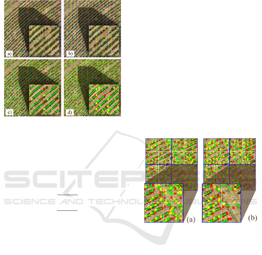
Figure 3: Overlap Strategy: a) image windowed with-

out overlap; b) image windowed with overlap of 25%;

c)Processed image windowed without overlap; d) Processed

image windowed with overlap of 25%.

The computation of the tiles coordinates can be

tricky. Therefore, we deﬁne two parameters. The ﬁrst

one β represents the size (in pixels) of the square tile.

The second parameter α represents the degree of over-

lap desired.

c = d

β(1 − α)

r = d

β(1 − α)

(1)

In order to compute the coordinates of each win-

dow we ﬁrst require to estimate the number of tiles

in each row and column. Equation 1 speciﬁes how to

compute the number of columns - c - and rows - r - for

a given image. It depends of the width - w - and height

- h - of the image as well as the size of the desired win-

dow and the degree of overlap. The ceil operator is

taken to ensure a round number of columns and rows

since there is a possibility the mosaicking of windows

will not ﬁt perfectly inside the image. In such cases

tiles located in the rightmost column and bottom row

will potentially be not squared and smaller in compar-

ison to the other tiles.

The coordinates of each tile can be computed us-

ing Equations 2. [x

] correspond to the upper left

coordinate of the window and [x

] to the bottom

right. Variables i and j are the row and column in-

dexes of the windows grid over the image. The win-

dowing strategy is depicted in Fig. 3.

(i) = i(β(1 − α)), 0 ≤ i ≤ c

( j) = j(β(1 − α)), 0 ≤ j ≤ r

(i) = x

(i) + β

( j) = y

( j) + β

(2)

A side effect of the tiling scheme is the introduc-

tion of undesired artifacts not pertaining to the plan-

tation lines. Such artifacts can be seen as noise and

therefore a post processing ﬁltering step is required.

2.3 Hough Transform and Post

Processing

Considering the coordinates of each tile, the method

proceeds by applying the Hough Transform. As out-

put, a set of lines (represented by its two end points)

is returned for each tile. The line segments can be

observed in Fig. 3 and 4.

Figure 4: Denoising example with 2 as index: a) Figure

without a denoising process; b) Figure with denoising algo-

rithm.

Although the overlap strategy solves the problem

of line discontinuity as side effect a number of ex-

traneous lines are produced. Therefore some ﬁlter-

ing is required as post processing in order to remove

such undesired lines. It happens in two stages: i)

inside each tile; and ii) using larger tiles with size

γ = ×1.5, ×2.0 or ×2.5 the size of the individual tiles,

γ is also called denoising index. The second stage is

necessary to further expunge erroneous segments. In

both stages the same set of steps are taken.

The noise removal starts by computing the angu-

lar coefﬁcient m = ∆

/∆

for all lines in a tile. All

coefﬁcients are then rounded to one decimal place.

The statistical mode is then computed for the angular

coefﬁcients and it is taken as the orientation tendency

for the tile. All lines are inspected for intersection and

in identifying such event all lines but the one closest

VISAPP 2018 - International Conference on Computer Vision Theory and Applications

456

to the tiles angular coefﬁcient mode are removed. Af-

terwards all remaining lines are inspected with regard

to the distance of its angular coefﬁcient to the mode.

Any line which differ from the mode for more than a

parameter δ are also removed. The difference should

be taken in absolute values. In our experiments δ was

set to 0.3 whose results are shown on Fig 4.

3 DATASETS AND

EXPERIMENTS

Eight distinct aerial images taken from a UAV named

sx2 (ﬁg. 5) were used in our experiments. During cap-

ture the the vehicle ﬂies between 100 and 150 meters

above the ground. It’s air speed must be at least 10

meters per second, not exceeding 15m/s. The UAV

is completely autonomous and can ﬂy up to 1.5 hours

nonstop. The ﬂight path is set to cover all analyzed

area. It is also conﬁgured that a snapshot of the plan-

tations is taken every 2 seconds. The RGB camera

used to take the pictures is a modiﬁed Canon S110.

Originally it can only capture red, green and blue

(RGB) frequencies, however to calculate the NDVI

the near-infrared spectrum is needed. Therefore, the

original optical ﬁlter is replaced for one that enables

the perception of the near-infrared channel, result-

ing in a near-infrared, green and blue (NIRGB) im-

age. For the purposes of this experiment, NIR was

taken as Red channel. In order to the results com-

parison, the images used in the tests are available in:

(http://www.facom.ufu.br/ mauricio/VISAPP2018/).

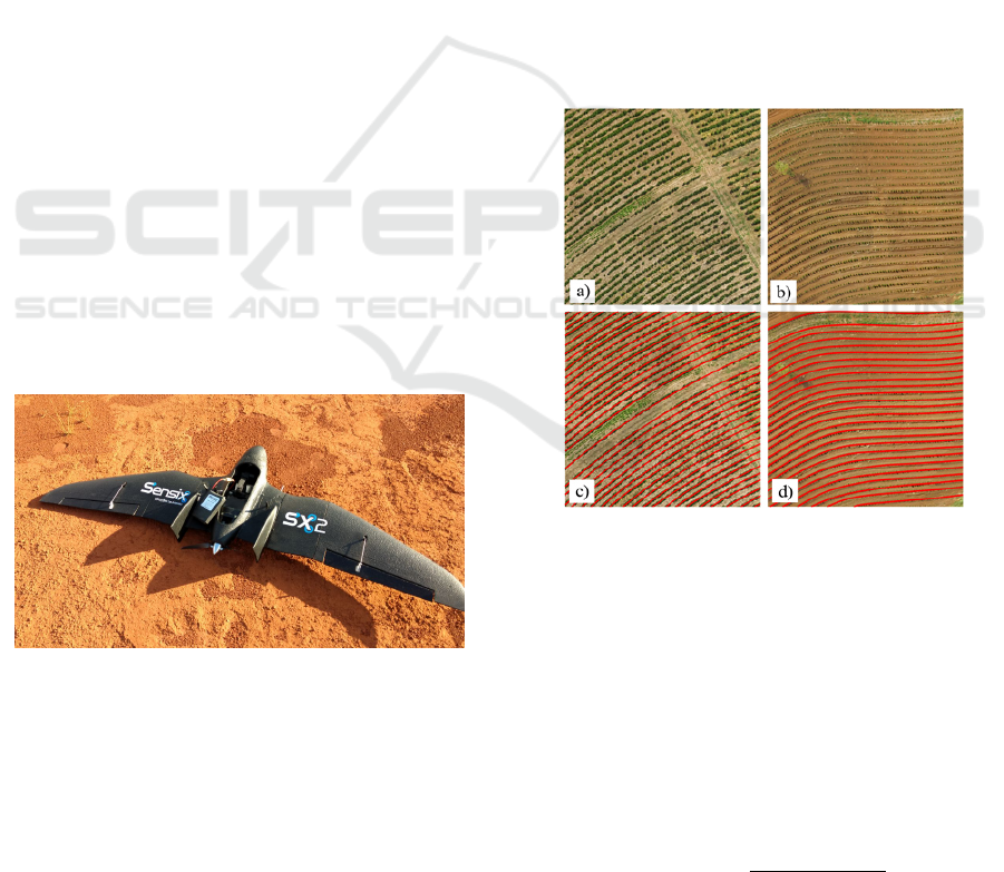
Figure 5: UAV utilized to capture crop images.

As previously presented, the proposed method de-

pends on three main parameters: size of tiles (β),

overlap percentage of (α) and denoising tile size (γ)

. In order to evaluate the performance of the proposed

algorithm in terms of the presented parameters, tests

were performed with different sets combining the val-

ues of β, α, and γ. The values used on those experi-

ments are presented by Table 1.

To evaluate the effectiveness of the proposed

methodology, the images used were taken from dif-

ferent coffee plantations and submitted to the pro-

posed algorithm. In order to assess the algorithm’s

accuracy under different commonly encountered con-

ditions, the images were taken with varying terrain,

atmospheric conditions and plant growth stages.

Each image had its ground truth manually gen-

erated by a specialist, who manually marked the in-

tended plantation rows. After applying the proposed

algorithm and obtaining a total of 36 variations from

each of the three images, the result was manually

evaluated considering its respective ground truth. The

crop lines were classiﬁed in three groups: a) in Green

segments of the plantation row correctly classiﬁed by

the algorithm; b) in Red were represented the seg-

ments not identiﬁed by the algorithm that actually are

part of the plantation row; and c) in Blue the seg-

ments identiﬁed by the algorithm that are not part of

the plantation row. Fig. 6-c,d shows the ground truth

generated prior to the application of the proposed al-

gorithm. Fig. 7 shows the manual classiﬁcation pro-

cedure after.

Figure 6: Data Set Example: (a) and (b) are two original

images; (c) and (d) represent the images after ground truth

deﬁnition.

The values presented on table 1 were combined

generating 36 combinations of the parameters α, β

and γ. For the images processed under each of such

parameter set, the accuracy rate was obtained by

the equation (3). The values of true-positive, true-

negative, false-positive and false-negative were ob-

tained manually by direct measurements against the

ground truth. A example of this process is presented

on Fig. 7.

accuracy =

T P

T P + FN + FP

(3)

In order to measure the accuracy rate, the Jaccard

Plantation Rows Identiﬁcation by Means of Image Tiling and Hough Transform

457

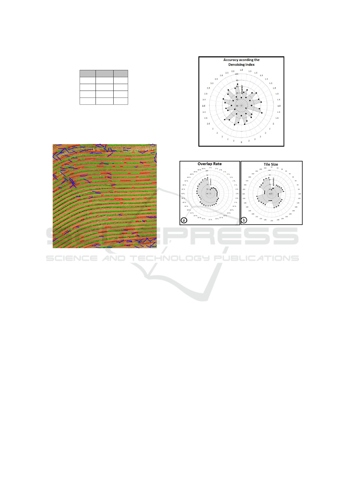
Table 1: Values tested for the variables used in the proposed

algorithm.

(β) (α) (γ)

50 0% 1.5

100 25% 2.0

150 48% 2.5

200 - -

Coefﬁcient was used, since this index disregard the

true-negative values, what in this case, represents all

the image area with no crop lines, which could com-

promise the results.

Figure 7: Accuracy Analysis Example: red line = False-

Negative, blue line = False-Positive and green lines = True-

Positive.

The accuracy rate achieved in the experiments was

associated with which one of the parameters evalu-

ated. The chart presented on Fig. 8 relate the accuracy

rate with the denoising index. According to data rep-

resented on this graphic, is impossible to determine

a relationship between the accuracy rate and the de-

noising index.

However, by considering the relationship between

the tile size and the overlap rate with the accuracy

rate, the dependence between this values was made

clear. Especially when considered the values of over-

lap rate (Fig. 9-a). Higher values of overlap rate pro-

duce better accuracy scores. Experimentally, overlaps

larger than 48% haven’t succeed in improve the re-

sults.

A curious behavior can be observed regarding the

tile size deﬁned by parameter (β). It is possible to

see on Fig. 9-b, that the results obtained ﬂuctuates.

To understand this result is important to realize that

each value of β tested was combined with two oth-

ers parameters as represented on Table 1. Thus, were

generated and tested nine sets of parameters for each

Figure 8: Results obtained with the denoising algorithm.

Figure 9: Polar plot of (a) Accuracy×Overlap rate, and (b)

Accuracy×Tile size.

value of β. For the design of the chart represented on

9-b the data were sorted by the values of β as the ﬁrst

criteria and by the overlap rate as the second criteria.

Thus is possible to realize that for the same values

of β the proposed algorithm achieve different accu-

racy values and they are totally dependent of the over-

lap rate value. The best results were obtained using

α = 0.48 and β = 200. Those values were then used

to apply the method on ﬁve other images in order to

test its reproductibility. It was possible to certify that

the average accuracy rate was maintained, with the

results on Table 2.

4 CONCLUSION

In this work were explored the application of Hough

Transform to extract plantation lines on UAV imaged

crop ﬁelds. In order to make it feasible were proposed

to tile the entire image into overlapped windows. This

approach accomplished to limit the information inside

each window to lines of manageable size which can

be considered locally straight making viable the use

of the Hough Transform. The overlapping windows

has shown to be a necessity in order to avoid discon-

tinuities in the plantation lines.

VISAPP 2018 - International Conference on Computer Vision Theory and Applications

458

Also a method were proposed to treat the un-

aligned lines generated by the proposed algorithm.

These lines were considered and treated in this work

as noise. Based on empiric analysis the technique de-

veloped prove itself a promising strategy to solve the

problem. It suggest future works in order to analyze

effectively the denoising algorithm proposed and as-

sess quantitatively their effectiveness.

Another interesting byproduct of the proposed ap-

proach is the possibility of parallelization. Each win-

dow is independent from one another making it ideal

to be implemented as a divide and conquer approach.

Considering that in production the size of the imaged

ﬁelds can be really large leading to possibly gigabytes

of image data, the post ﬂight processing can take con-

siderable time. By parallelizing the process, the UAV

companies doing agricultural survey are enabled to

deliver the ﬁnal processing result in a fraction of the

usual time.

ACKNOWLEDGMENT

The authors would like to thank the company Sensix

Inovac¸

oes em Drones Ltda (http://sensix.com.br) for

providing the images used in the tests.

REFERENCES

AUVSI (2013). The economic impact of unmanned aircraft

systems integration in the united states march. Eco-

nomic report, Association for Unmanned Vehicle Sys-

tems International, Washington DC,.

Ballard, D. H. (1981). Generalizing the hough transform to

detect arbitrary shapes. Pattern Recognition, 13(Issue

2):111–122. doi:10.1016/0031-3203(81)90009-1.

Blackmer, T. M. and Schepers, J. S. (1996). Aerial pho-

tography to detect nitrogen stress in corn. Journal of

Plant Physiology, 148:440–444. doi:10.1016/S0176-

1617(96)80277-X.

Garc

ıa-Santill

an, I., Guerrero, J. M., Montalvo, M., and

Pajares, G. (2017). Curved and straight crop row

detection by accumulation of green pixels from

images in maize ﬁelds. Precision Agriculture.

doi:10.1007/s11119-016-9494-1.

Hough, P. (1962). Method and Means for Recognizing

Complex Patterns. U.S. Patent 3.069.654.

Illingworth, J. and Kittler, J. (1988). A survey of the hough

transform. Computer Vision, Graphics, and Image

Processing, 44(Issue 1):87–116. doi:10.1016/S0734-

189X(88)80033-1.

Kataoka, T., Kaneko, T., Okamoto, H., and Hata, S.

(2003). Crop growth estimation system using ma-

chine vision. In Advanced Intelligent Mechatronics.

doi:10.1109/AIM.2003.1225492.

Lee, I.-K. (2000). Curve reconstruction from unorganized

points. Computer Aided Geometric Design, 17(Issue

2):161–177. doi:10.1016/S0167-8396(99)00044-8.

Leemans, V. and Destain, M.-F. (2006). Line cluster de-

tection using a variant of the hough transform for cul-

ture row localisation. Image and Video Computing,

24:541–550.

Ramesh, K. N., Omkar, N., Meenavathi, M. B., and Rekha,

V. (2016). Detection of row in agricultural crop im-

ages acquired by remore sensing from a uav. Inter-

national Journal of Graphics and Signal Processing,

11:25–31.

Ronghua, J. and Lijun, L. (2011). Crop-row detection algo-

rithm based on random hough transformation. Math-

ematical and Computer Modelling, 54:1016–1020.

Sankaran, S., Khot, L. R., et al. (2015). Low-

altitude, high-resolution aerial imaging systems

for row and ﬁeld crop phenotyping: A re-

view. European Journal of Agronomy, 70:112–123.

doi:10.1016/j.eja.2015.07.004.

Søgaard, H. T. and Olsen, H. J. (2003). Determination of

crop rows by image analysis without segmentation.

Computers and Electronics in Agriculture, 38(Issue

2):141–158. doi:10.1016/S0168-1699(02)00140-0.

Turner, J., Kenkel, P., Holcomb, R. B., and Arnall, B.

(2016). Economic potential of unmanned aircraft in

agricultural and rural electric cooperatives. In 2016

Annual Meeting of Southern Agricultural Economics

Association, number 230047, page 18, San Antonio,

Texas.

Plantation Rows Identiﬁcation by Means of Image Tiling and Hough Transform

459