Hydrodynamic Adaptive Routing Algorithm for Unstable Sensor

Networks with a Tsunami Model of Acute Events

Ekaterina V. Aleksandrova

1,2

and Vladimir A. Bashkin

P. G. Demidov Yaroslavl State University, 150003, Sovetskaja ul., 14, Yaroslavl, Russia

Yaroslavl State Technical University, 150023, Moskovsky pr., 88, Yaroslavl, Russia

Keywords:

Unstable Sensor Network, Adaptive Routing, Acute Event, Hydrodynamic Model, Tsunami Model, Seismic

Wave.

Abstract:

An algorithm of adaptive multi-path routing in unstable sensor networks with frequent reconﬁgurations is

presented. The model is based on the discrete imitation of water streams and water waves in the network of

river-connected reservoirs. The hydrodynamic phenomena of water currents, riverbed erosion and sediments

deposition are used as convenient models of different algorithmic features of the routing scheme. Acute

network events (topology changes, node failures, gateway migrations etc) are treated by imitating of such

natural phenomena as underwater seismic activities and surface tsunami waves.

1 INTRODUCTION

Nature-inspired heuristics such as directed diffusion

(Intanagowiwat et al., 2000), gradient-based routing

(Schurgers and Srivastava, 2001), thermal ﬁeld rout-

ing (Baumann et al., 2008) and ant colony optimiza-

tion (DiCaro and Dorigo, 1998) have shown to be a

good technique for developing adaptive routing algo-

rithms for sensor networks.

In (Aleksandrova and Bashkin, 2016) we de-

scribed a novel approach, based on the discrete imi-

tation of water ﬂow in the network of water reservoirs

(nodes), connected by rivers (links). The ﬂow direc-

tion (data route direction) depends on the difference

of absolute water level (queue length) in neighboring

reservoirs. Some reservoirs may have additional un-

derwater springs (data sources), some others are wa-

ter drains (sinks, gateways). Different reservoirs may

have different absolute bottom levels, drains are al-

ways the deepest in the network. Constant transit wa-

ter ﬂow deepens reservoirs that are located closer to

drains than others - a physical phenomenon, called

riverbed erosion (we use it as an adaptive preferred

routing). On the other hand, constant absence of wa-

ter outﬂow together with high water level imply de-

position of sediments and hence the rise of the bottom

level in the node (adaptive routing penalization).

The key features of our algorithm are its sim-

ple physical model and easy-to-understand multifac-

tor structure. It is possible to reconﬁgure a large

set of “real-world” parameters: frame size (“wa-

ter density”), link speed (“river width”), reconﬁg-

uration rates (“soil density” and “soil condensation

rate”), buffer speed/volume effectiveness (“surface

area of the reservoir”), etc. Moreover, the clear phys-

ical model can be easily enhanced with additional

naturally-inspired phenomena, such as surface waves

(data interference and multicast storms) and deepwa-

ter currents (control data ﬂows). We believe that the

proposed concept may be used as a general base for a

wide range of proactive routing algorithms.

In this paper we present a modiﬁcation of basic

algorithm for unstable networks with more frequent

acute events such as topology changes, node failures,

gateway migrations etc. Intuitively, all these events

require some abrupt changes in the routing scheme,

that is based primarily on the “water surface level” in

different nodes. Here we try to incorporate into our

model the closest natural phenomenon – a tsunami.

A tsunami is a natural “procedure” that stabilizes

water currents and waves after underwater seismic ac-

tivities: quakes, landslides and volcanic eruptions. In

our model we have an analogue of seabed relief –

the map of bottom levels of all nodes. So there is a

straightforward way to trigger the “tsunami” – it is

sufﬁcient to apply some appropriate changes to the

bottom levels of nodes, adjacent to the node with an

acute “catastrophic” events (to trigger an appropriate

Aleksandrova, E. and Bashkin, V.

Hydrodynamic Adaptive Routing Algorithm for Unstable Sensor Networks with a Tsunami Model of Acute Events.

DOI: 10.5220/0006655901410146

In Proceedings of the 7th International Conference on Sensor Networks (SENSORNETS 2018), pages 141-146

ISBN: 978-989-758-284-4

141

“landslide” or “eruption”).

There may be different heuristics of seismic ef-

fects. In this paper we present a very simple concept:

a node monitors the bottom levels of its neighbors and

in the case of abrupt changes of the mean value ad-

justs its own bottom level. This can be interpreted as a

certain ﬂowability of a sea bottom soil. Surprizingly,

such simple heuristic allows to adequately react to a

wide range of target events. For example, after the

shutdown of an important transit node (or a gateway)

we can observe both a seismic wave on the seabed

and a tsunami on the surface. The new model also

allows to accelerate the global balancing. For exam-

ple, after connection of two previously disconnected

subnets we can observe both landslides on the bottom

and waves on the surface, quickly reconﬁguring the

routing “map” of an entire network.

The paper is organized as follows. In Section 2

the routing algorithm is presented. Informal examples

are given. We also consider and evaluate some key

properties of an algorithm. In Section 3 we brieﬂy

describe preliminary results of imitational modeling.

Section 4 contains some conclusions.

2 ROUTING ALGORITHM

2.1 Informal Model – No Acute Events

In this subsection we describe the basic principles of

our hydrodinamic model for unstable sensor neworks,

as it was given in (Aleksandrova and Bashkin, 2016).

This concept is quite ﬂexible and tuneable and can

be applied to a wide range of situations. However,

in our opinion, it is best suited for unstable networks

with a relatively “smooth” dynamics of changes (re-

locating nodes, energy consumption, moving subject

of surveillance, etc). The novel enhancement of this

algorithm, better suited for nets with more frequent

acute events will be given in a Subsection 2.2.

All hosts are synchronized, the global time is

quantiﬁed in “rounds”. The frame size is ﬁxed.

A network consists of a ﬁxed ﬁnite set of n hosts

H = {h

,... ,h

} and a variable ﬁnite set L of sym-

metric links. In any conﬁguration (at any moment of

time), if L = {l

,. .. ,l

} then for all i ∈ {1,. .. ,m} we

have l

= (h,h

′

) with h,h

′

∈ H and h ̸= h

′

Each link l has its maximal transfer rate Width(l)

(“river width”), measured in “frames per round” (fpr).

Each host h has buffer effectiveness Area(h), mea-

sured in frames (“surface area of the reservoir”). It

also has four variable attributes: Top(h) — the ab-

solute “water surface level” (in frames), i.e. “Top

→

←

→

1→

←

→

Figure 1: Balancing queue lengths (“water waves stabiliza-

tion”).

level”; Low(h) — the absolute “bottom surface level”

(in frames), i.e. “Low level”; In(h) — the incom-

ing dataﬂow rate (in fpr, nonnegative); Out(h) —

the outgoing dataﬂow rate (in fpr, nonnegative). If

Out(h) > 0 then h is a sink (a drain) and we set

Low(h) = −n (hence all sinks are the deepest sites).

For the sake of shortness we describe here the sim-

plest variant of our model: all links have the same

maximal transfer rate (3 fpr in the examples), all hosts

have the same buffer effectiveness (1 frame in the fol-

lowing examples). Transfer rates and buffer sizes are

constant and never change (in contrast to water sur-

face level and bottom level, which are affected by

wave propagation and riverbed erosion).

Algorithm is proactive: we deﬁne the behavior of

a single node. The particular node h possesses all the

information about its local conﬁguration and also the

top and low levels of all its neighboring nodes (nodes

with direct links to h). For a node h we denote the set

of its neighbors by N(h). Hence, for any h

′

∈ N(h)

the local node h knows values Top(h

′

) and Low(h

′

The model is based on several physical principles.

The ﬁrst law deﬁnes the way, in which the exces-

sive frames (“extra water”) are distributed (“spread”)

among adjacent nodes (“on the surface”). The infor-

mal rule is very simple: we let the water ﬂow to the

neighboring reservoirs with the lower water surface

level (frame-by-frame, starting from the node with the

lowest level, without exceeding the capacity of links

and reservoirs), while there exists such reservoirs.

An example is given in Fig. 1. Here we depict a

time sequence (from left to right) of 5 successive con-

ﬁgurations (between time rounds) of a simple net. A

net in the example is a chain of 5 nodes, without in-

going and outgoing external links (a chain of 5 reser-

voirs without springs and sinks). In the initial conﬁg-

uration the ﬁrst (from the left) node has 7 dataframes

(depicted by rounded rectangles), the second — 3, the

third — 9, and so on. The bottom levels are the same,

so the water surface levels are also 7–2–9–4–2. Each

round includes a set of data movements, depicted by

weighted arrows. For example, during the ﬁrst round

2 frames moves from node #1 to node #2, 3 frames

from #3 to #2, 1 frame from #3 to #4 and 1 from #4

to #5. The “water levels” are stabilized after 4 rounds

– to the global conﬁguration 6–6–5–4–4. Now “the

water is calm”.

The next example (Fig. 2) illustrates the same

SENSORNETS 2018 - 7th International Conference on Sensor Networks

142

←

→

←

→

←

→

←

→

←

→

←

→

←

→

←

→

←

→

←

→

←

→

←

→

←

→

←

→

←

1 fpr (in)

←

1 fpr (out)

←

2 fpr (in)

←

2 fpr (out)

Net configuration:

Figure 2: Balancing output (“water currents stabilization”).

→

Figure 3: Adaptive routing I (“riverbed erosion”).

physical law, but in a more comprehensive situation:

a net with incoming and outgoing data streams. Here

nodes #1 and #4 are gateways with maximal outgoing

transmission speed 2 fpr and 1 fpr respectively, nodes

#2 and #3 are sensors (data generators) with incom-

ing streams of 1 fpr and 2 fpr. As it can be seen, the

ﬂow directions and rates stabilize after 14 rounds. The

physical analogy is the formation of stable currents in

the water system with constant inﬂow and outﬂow.

The other physical phenomenon is the erosion

of the river bottom. The more stable and powerful

stream produces the stronger soil erosion and hence

the resulting channel becomes a “mainstream” for fu-

ture transmissions. An example is given in Fig. 3.

Here we can see a chain of four nodes with a sin-

gle gateway (#4). The stream gradually cuts the bot-

tom “edge”, forming the slopes. The basic rule is

quite simple: the bottom level of current node is low-

ered if the accepting neighbor had surface level lower

than current node’s bottom level (“water is slopping

over”) and the corresponding ﬂow is strong enough —

i.e., the number of moving frames exceeds a speciﬁc

ErosionParameter (we set it to 2 in the examples).

And the third key physical process is a deposi-

tion of sediments on the river bottom. If the ﬂow

→

←

→

Figure 4: Adaptive routing II (“deposition of sediments”).

rate is low and the water column is high then the

bottom level rises. In our model we simplify both

these factors (time and volume) into a single “sedi-

ments counter” Sediments(h) that is incremented at

each round by a number of dataframes that lay immo-

bile in the node h. If any number of frames moves out

of the node then the counter is reset. If the counter

value exceeds a speciﬁc SedimentsParameter (we set

it to 6 in the examples) then the bottom level is raised

(and the counter is reset). An example is given in

Fig. 4. Here the counter values are depicted under the

corresponding nodes. With the lapse of time coun-

ters for nodes #1 and #2 are growing (the second one

grows two times faster because of 2 dataframes lo-

cated). So the bottom levels begin to rise and eventu-

ally the slopes are formed.

2.2 Informal Model of Acute Events

In this paper we want to show that the basic model

can be transparently enhanced to better handle such

acute events as node disconnection/reconnection and

gateway start/shutdown. Note that the causes of these

events may be of a different nature: fast moving

nodes, battery discharge, signal obstacles etc.

In fact, the basic model already handles all these

events quite successfully. For example, the switching-

on of a new gateway will cause the creation of new

riverbeds and (possibly) the silting of some old ones.

However, the reaction time may be substantially im-

proved by forced “deepening of the bottom” in some

of neighboring nodes. The closest natural models for

these events are quakes, landslides and other similar

seismic processes occuring at the “ocean ﬂoor”.

The main new idea of the algorithm is to model

a tsunami in the ocean. Tsunami often occurs as a

result of a sharp rise or fall of the sea bottom (over a

large area). In our model we have a bottom level —

so “seismic” features can be easily implemented.

Let’s consider several types of “catastrophic”

events in the sensor network and variants of their reso-

lution under the new scheme (with “earthquakes” and

“tsunami”). All situations are considered from the

point of view of a particular node:

Hydrodynamic Adaptive Routing Algorithm for Unstable Sensor Networks with a Tsunami Model of Acute Events

143

• The disappearance of a neighbor node whose bot-

tom level was below our bottom level (i.e., this

node in the recent past most likely was receiving

packets from us rather than sending them to us).

We believe that in the neighborhood a new “is-

land” was formed (“an earthquake has raised the

bottom”), so in our location the bottom level also

should slightly rise (and so a tsunami is formed).

How much to raise the bottom is determined by

the heuristic (see below).

• The disappearance of a neighbor node, which

transmitted packets to us (the level of its bottom

was higher than ours). We believe that the place of

the missing node has a “pit”, so we lower our local

level of the bottom a bit. A kind of a “whirlpool”

may be formed, making the node more attractive.

• The emergence of a neighbor node (consider both

a lower and a higher bottom). It’s one thing if

the node is completely new and just emerged from

nowhere, then, in principle, it can simply be em-

bedded into a network with an average bottom

value in a given “region” (taking the arithmetic

mean of the neighbors’ levels). Another thing is

if the node is already participating in some other

subnetwork with established levels (perhaps very

different from ours). Consider only the second sit-

uation. We propose to speed up the process of

leveling the bottom levels in subnets (raise if we

had lower, or deepen if we had higher ones), so

that the streams stabilize faster. In nature, this can

be compared with the rapid destruction of a thin

“dam” between two reservoirs with different lev-

els of bottom and water: simultaneously there will

be (1) a “waterfall” from a reservoir with a higher

water level to another one and (2) the landslide in

the area of the destroyed dam wall from the shal-

low reservoir to the deeper one.

•

Gateway switching off. Even in the basic ver-

sion of our algorithm there will be a fairly fast

(for a few time rounds) increase in the water level

at the former gateway node and all its neighbors

(the water “pouring”), so a kind of a big wave

will be formed. However, the bottom level will

change very slowly, because initially the gateway

was very deep. We propose to accelerate this pro-

cess: to raise the water level substantially and

rapidly by raising the bottom level to an average

value among all neighbors. Tsunami then will be

higher and more stable.

• Enabling the gateway role on the node. The bot-

tom level at the gateway instantly becomes very

low. For a few time rounds the water level will

drop at the gateway and all its neighbors and there

–

Figure 5: Acute event I — receiving node occlusion (“seis-

mic wave” and subsequent “tsunami”).

–

Figure 6: Acute event II — sending node shutdown (“land-

slide” and subsequent “whirlpool”).

→

Figure 7: Acute event III — connecting two subnets with

different levels (“landslide” and “waterfall”).

will be something like waves converging to a new

sink (a “whirlpool”). We speed up the process

by substantially deepening the bottom level at the

neighbors (“landslides” from the slopes).

Thus, the beneﬁts of the introduction of the

“tsunami” are clearly visible. The problem is to come

up with an appropriate heuristic. The difﬁculty here

is that there can be several problematic neighbors. It

is necessary to take into account the possibility of the

emergence of various “catastrophic” changes for sev-

eral neighbors at once. We propose a simple solution:

to monitor the arithmetic mean of the bottom levels

of all neighbors. If the change is substantial (exceeds

some parameter) then we apply the same change to

our bottom level. Surprisingly, this simple heuristics

is adequate for all considered types of acute events.

Some examples are given below. We consider

the same chain-like topology as in the previous sub-

section, with simplest transfer rates and buffer sizes.

Moreover, for the sake of shortness we do not recalcu-

late water streams – only the bottom level dynamics

(“seismic activity”) is considered.

Consider Fig. 5. Here we depict a time sequence

of a net with a disconnected sink node (#1). At the

second round the node #2 ﬁnds out that the average

bottom level is raised from 2 to 4 (i.e. the delta is +2),

and hence at the third round it “lifts” its own bottom

from 4 to 6. Now, the node #3 is also affected (+1 at

the fourth round) – a fading seismic wave is formed.

At Fig. 6 we can see an opposite process – a land-

slide after the shutdown of an active sending node.

Here the node #2 discovers a gap and crumbles itself.

Fig. 7 depicts the emergence of a neighbor node

with a different bottom level.

SENSORNETS 2018 - 7th International Conference on Sensor Networks

144

2.3 Formal Deﬁnition

All nodes behave independently, the scheme is purely

proactive. We deﬁne a behavior of a single node

throughout a single time round. At the starting

moment of the round the node h knows every-

thing about itself (Top(h),Low(h), In(h), Out(h) and

Sediments(h)) and also knows levels and link band-

width of all it’s neighbors: Top(h

′

),Low(h

′

) and

Width(h,h

′

) for any h

′

∈ N(h).

An algorithm (in pseudocode) is given below.

For simplicity we denote N(h), In(h), Out(h) and

Sediments(h) by N,In,Out and Sediments.

Algorithm: 1 Behaviour of a single node h during a single

time round.

Constants (tuning parameters):

ErosionParam, SedimentsParam

: Nat

SeismicParam,IOFlowParam

: Nat

Persistent variables:

: set of Node

Top,Low

: map of (Node -> Int)

Width

: map of ((Node * Node) -> Nat)

In, Out,Sediments

: Nat

Round (local) variables:

h’ : Node

N’, Receivers, Above : set of Node

BufferTo : map of (Node -> Nat)

BufferOut, LowAvg, LowAvgNew : Nat

IOFlowDelta, LowAvgDelta : Int

Step 1

/* Computations */

N’, Receivers, Above :=

∅

BufferOut := 0

foreach h

′

∈ N let

BufferTo[h’] := 0

BufferOut :=

min{Out,Top[h] − Low[h]}

Top[h]

-BufferOut

Iteration

if Top[h]

Low[h] goto

Final

Above :=

{x ∈ N : Top[x] > Top[h] + 1}

N’ :=

N \

Receivers

Above

N’

= ∅ goto

Final

take

h’

from N

′

s.t. Top[

h’

] = min

x∈N

′

Top[x]

BufferTo[h’] :=

min{ (Top[h] − Top[

h’

]) div 2,

Top[h] − Low[h],

Width[h,

h’

] }

Top[h]

Top[h] − Bu f f erTo

[h’]

Receivers := Receivers

∪ {h

′

}

goto

Iteration

Final :

Receivers

̸= ∅

begin

take h

′

from

Receivers

s.t.

Low[h

′

] < Low[h] and

BufferTo[

′

]

≥ ErosionParam

if h

′

̸=

NULL

begin

Low[h]

Low[h] − 1

Top[h]

Top[h] − 1

end

Sediments

:= 0

end

else

begin

Sediments

(Top[h] − Low[h])

if Sediments

SedimentsParam

begin

Low[h]

Low[h] + 1

Top[h]

Top[h] + 1

Sediments

:= 0

end

Step 2

/* Data communications */

•

Try to

send

BufferOut dataframes to the

local gateway. In the case of failure

increase

Top[h]

accordingly.

•

Try to

send Bu f f erTo[h

′

]

dataframes to each

neighbor

′

In the case of failure increase

Top[h]

accordingly.

• Receive

some dataframes from each neighbor,

increase

Top[h]

accordingly.

• Receive In

dataframes from the local sensor,

increase

Top[h]

accordingly.

Step 3

/* Control communications */

(a)

Estimate

the new values of incoming and

outgoing flow (from the sensor and to the

local gateway)

InNew

and

OutNew

for the

next round.

IODelta := (Out − In) − (OutNew − InNew)

if |IODelta| > IOFlowParam

begin

Low[h] := Low[h] + IODelta

Top[h] := Top[h] + IODelta

end

In := InNew

;

Out := OutNew

(b)

Send

the new

Top[h]

and

Low[h]

to the

neighbors.

(c)

LowAvg := (

∑

′

∈N

Low[h

′

])/|N|

(d)

Receive

the new

Top[h

′

],Low[h

′

]

and

Width[h, h

′

]

from each neighbor

′

, calculate the value

for the next round.

(e)

LowAvgNew := (

∑

′

∈N

Low[h

′

])/|N|

LowDel ta := LowAvgNew − LowAvg

LowAvg := LowAvgNew

if |LowDelta| > SeismicParam

begin

Low[h] := Low[h] + LowDelta

Top[h] := Top[h] + LowDelta

end

Note that substeps of Step 2 may be executed in

any order (or in parallel). The same is not true for

the substeps of Step 3 ((c), (d), (e) must follow one

another sequentially). A substep 3(a) allows to react

to the abrupt changes of the dataﬂows from the lo-

cal sensor and to the outer network (through the local

gateway). This includes sensor activation, gateway

shutdown etc.

Hydrodynamic Adaptive Routing Algorithm for Unstable Sensor Networks with a Tsunami Model of Acute Events

145

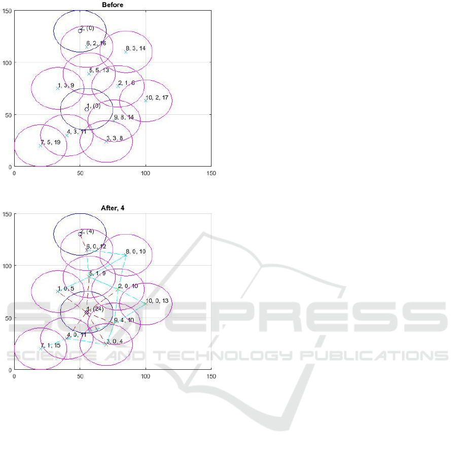
Figure 8: Initial conﬁguration.

Figure 9: Conﬁguration after 4 rounds.

2.4 Modeling

An example of routing scheme modeling is given in

Fig. 8 and Fig. 9. Here a simple sensor network

is modeled in MATLAB, consisting of eight sensors

(denoted by X-crosses) and two gateways (denoted by

small circles). Large circle denote the “transmitting

power” of the node. Each ordinary node is labeled

by a triple (node number, bottom level, surface level).

Gateways in this model are simple and can only re-

ceive frames. They are labeled by (sink number, re-

ceived frames). All frames will reach the gateways in

30 rounds.

The experiments were carried out in MATLAB for

the random arrangement of a ﬁxed number of nodes.

Preliminary results show satisfactory routing and load

balancing rates.

3 CONCLUSION

Many approaches have been proposed for multiple-

path routing in sensor networks. Among them

there are a number of gradient-based and physi-

cally/biologically inspired algorithms. For a short

survey see (Aleksandrova and Bashkin, 2016).

The proposed routing algorithm is adaptive and scal-

able. We also believe that it can be further improved

by taking into consideration other important aspects

such as energy consumption. The key feature of the

model is its simple and natural interpretation, allow-

ing to implement purely “physical” reasoning without

any artiﬁcial heuristics.

We will explore the model in our future work.

In particular, further research will be concentrated

on the comparative study of our scheme with other

known routing algorithms in different network conﬁg-

urations. Another direction is the implementation of

new routing concepts in hardware and software wire-

less mesh network controllers (Sokolov et al., 2016).

ACKNOWLEDGEMENTS

This work was partially supported by Russian Fund

for Basic Research (project 17-07-00823) and YarSU

(project AAAA-A16-116070610022-6).

REFERENCES

Aleksandrova, E. V. and Bashkin, V. A. (2016). Hydrody-

namic model of adaptive routing for large-scale unsta-

ble sensor networks. In SIBCON, Int. Siberian Conf.

on Control and Communications. IEEE.

Baumann, R., Heimlicher, S., and Plattner, B. (2008). Rout-

ing in large-scale wireless mesh networks using tem-

perature ﬁelds. IEEE Network, 22(1):25–31.

DiCaro, G. and Dorigo, M. (1998). Antnet: Distributed stig-

mergetic control for communication networks. Jour-

nal of Artiﬁcial Intelligence Research, 9:317–365.

Intanagowiwat, C., Govindan, R., and Estrin, D. (2000).

Directed diffusion: A scalable and robust communi-

cation paradigm for sensor networks. In MOBICOM,

6th Int. Conf. on Mobile Comp., pages 56–67. ACM.

Schurgers, C. and Srivastava, M. B. (2001). Energy efﬁ-

cient routing in wireless sensor networks. In MIL-

COM, Military Comm. Conf., pages 357–361.

Sokolov, V. A., Korsakov, S. V., Smirnov, A. V., Bashkin,

V. A., and Nikitin, E. S. (2016). Instrumental support-

ing system for developing and analysis of software-

deﬁned networks of mobile objects. Automatic Con-

trol and Computer Sciences, 50(7):536–545.

SENSORNETS 2018 - 7th International Conference on Sensor Networks

146