Solving the Flight Radius Problem
Assia Kamal Idrissi
1,2
, Arnaud Malapert
1
and R
´
emi Jolin
2
1
Universit
´
e C
ˆ
ote d’Azur, CNRS, I3S, Sophia Antipolis, France
2
Milanamos, 1047 route des Dolines, 06900 Sophia Antipolis, France
Keywords:
Flight Radius Problem, Route Network Development, Airline Schedule Design, Shortest Path Algorithm.
Abstract:
In this article, we present the flight radius problem on the condensed flight network. The problem is derived
from a decision tool for airline managers to analyze and simulate a new market. It concerns the network
design and visualization when allocating a new flight. The flight radius problem consists in finding routes
passing through a specific flight that represent business opportunities regarding time and cost criteria. It is
formulated as finding a maximal subgraph of nodes belonging to routes accepted by a regret function. The
regret is defined as a function of the optimal values of the time and cost criteria. In practice, the condensed
flight network is stored in a graph database Neo4j. First, we propose a query based on available procedures
in the database. Second, we propose a method that uses the regret function to speed up the successive calls to
Dijkstra algorithm. Results on a set of real-world instances with different flights (Hub & Spoke) and regret
function parameters demonstrate that the algorithm is more efficient than the query and meets real-world
response time constraints.
1 INTRODUCTION
The air transportation industry has evolved rapidly
over the last years. The growth of air passenger de-
mands has pushed airlines to enhance their quality of
service. The airlines should focus on the route net-
work development which is considered as the initial
problem addressed by the airlines. It aims to deter-
mine a set of routes to be operated in an airline’s net-
work. It takes passengers demand, airport and air-
craft characteristics, and then generate a set of origin-
destination pairs (OD) to serve, the schedule design
problem aims to define the frequency and departure
time of each flight. The airline planning process starts
from the fleet planning that involves aircraft acquisi-
tion, passing by the route network development and
schedule design to airline flight operations, such as
pricing policies and marketing (Barnhart et al., 2003).
The fleet planning consists to define type of aircraft
to acquire, when and how many of each. The pro-
cess begins more than three years in advance of flight
departure.
Airlines have the choice to create a new route to
serve a destination, this new route provides connect-
ing traffic to other flights, or to increase/decrease the
frequency of existing routes. The first requires the
route network development problem and the schedule
design problem which demand a lot of investment.
While in the second, the airline network already ex-
ists. The problem of allocating a new flight is related
to these problems. The problem consists of determin-
ing an (OD) pair to serve and then choose flight sched-
ules with respect to the quality of service index (QSI)
model. QSI is a market share model used by most air-
lines to estimate their part of the market (Jacobs et al.,
2012). We define a flight by three attributes: Origin-
Destination (OD) pair (an OD pair is a couple of air-
ports), arrival/departure time and aircraft type. We
distinguish between three different types of flights: A
non-stop flight is a single flight with no intermediate
stops. It is the preferred choice of most passengers.
In the absence of such flights, passengers must take
either a direct flight or a connecting flight. A direct
flight is operated by the same aircraft and includes at
least one stop. A connecting flight is a flight where
passengers have to change of aircraft in a hub. A
route is a sequence of flights with unique flight num-
bers that begins at the origin airport and ends at the
destination airport (Hall, 2012).
The problem of allocating a new flight evokes de-
sign and visualization of the airline’s network. How-
ever, the network is so large that it cannot be visu-
alized. Thus, we proposed the flight radius problem
which is related to the route network development
304
Idrissi, A., Malapert, A. and Jolin, R.
Solving the Flight Radius Problem.
DOI: 10.5220/0006654003040311
In Proceedings of the 7th International Conference on Operations Research and Enterprise Systems (ICORES 2018), pages 304-311
ISBN: 978-989-758-285-1
Copyright © 2018 by SCITEPRESS – Science and Technology Publications, Lda. All rights reserved

problem. This problem consists in finding only in-
teresting airports with respect to a specific flight re-
garding the QSI criteria. Cost and time are the major
QSI criteria. Besides, the regret criterion is compared
to the optimal time or optimal cost. The main idea
of the flight radius problem is to locate in the net-
work what routes, passing through a specific flight,
and represent business opportunities that are attrac-
tive to the passengers according to different prefer-
ences. The choice depends on the passengers since
they have different preferences over the criteria, and
the type of flight is one of these criteria. For this rea-
son, these preferences should be taken into considera-
tion in this problem; it is modeled by the regret func-
tion. The function aims to model the regret compared
to the optimal value of cost or time. The visualization
is a simple way to remove the irrelevant routes. Since
the airline network exists already, our aim is to filter
the network and keep only important routes passing
through this flight. For this reason, we omit the sched-
ule design by working on the condensed flight net-
work (see Section 4). In such network, we just con-
sider the transfer time without checking if the route
is viable. Hence, for an airline managers, what is the
relevant sub-network related to a given flight? What
are the passengers origins and destinations?
The flight radius problem is formulated as a prob-
lem of finding a maximal subgraph in terms of nodes.
We constructed the condensed flight network from the
company flight database using the time-independent
approach and stored it in the graph database Neo4j
since the current NoSQL database presents some limits
(Neo4j, 2017). The problem can be solved using the
shortest path algorithms to find the maximal subgraph
of the graph in terms of nodes. The output subgraph
contains nodes whose paths respect the regret func-
tion, and passing through the specific arc.
This problem is derived from the application de-
veloped by the company that has developed a deci-
sion tool for airline managers to analyze and sim-
ulate a new market using QSI models. We are in-
terested to simulate a new market. Given a specific
flight, the process starts by finding important airports
whose routes pass by the specific flight in terms of
QSI criteria, and then estimate market share for each
route. The solution proposed is to reduce the number
of routes before applying QSI models.
This paper is organized as follows. Section 2 in-
troduces some definitions of graph theory and flight
timetables. In Section 3, we review related work of
the air scheduling problems, transportation networks,
and shortest path algorithms. Section 4 describes the
condensed flight network. Section 5 gives our for-
mulation of the flight radius problem, and its proper-
ties. Section 6 describes methods proposed to solve
the flight radius problem. Section 7 is dedicated to
experiments.
2 PRELIMINARIES
Graph Theory. A graph G is a tuple G = (V, E)
consisting of a finite set V of nodes or vertices and a
set E ⊆ V ×V of arcs which are ordered pairs (u,v) if
the graph is directed. The node u is called the tail of
the edge, and v is called the head. Each arc (u,v) ∈ E
has an associated non-negative weight w(u, v). We de-
fine |V | = n, the order of the graph as the number of
nodes meanwhile |E| = m its size. In a directed graph,
the arcs point from one node to another. For instance,
airline networks are weighted directed graphs where
the weights represent the prices or the duration of the
flight. A direct flight from one city to another does
not necessarily imply that there is also a direct return
flight. A subgraph G
0
= (V
0
,E
0
) of a graph G where
V
0
is a subset of V and E
0
is a subset of E. A path is
a sequence of nodes {v
1
,v
2
,..., v
k
} such that for each
1 ≤ i < k condition (v
i
,v
i+1
) ∈ E holds. If addition-
ally v
1
= v
k
, then the path is a cycle. The length of
a path is the sum of its edge weights along the path
and is denoted by: l(P) :=
∑
k−1
i=1
w(v
i
,v
i+1
). By ex-
tension, we define l
?
(s,t) for a given pair of vertices,
the length of the shortest path starting at s and ending
at t. A path in G is called elementary if no vertex oc-
curs more than once. A graph G is connected if there
exists a path joining any two vertices. A transporta-
tion network should be a connected graph.
Flight Timetables. In this study we restrict to flight
networks that rely on timetables. A flight timetable is
defined by a tuple (C , A, F , T ) where A is a set of air-
ports, F is a set of flights, T is the periodicity of the
timetable, and C is a set of elementary connections
(Pajor, 2009). An elementary connection c ∈ C is a
tuple c = ( f , o, d,t
s
,t
e
) which represents flight f ∈ F
departing from the airport o ∈ A at t
s
< T and arriv-
ing at the airport d ∈ A in time t
e
< T . Concretely,
an elementary connection corresponds to an event in
the timetable. A passenger trip (c
1
,c
2
,. .. ,c
n−1
,c
n
)
is a sequence of elementary connections, with the ori-
gin of an elementary connection the same as the des-
tination of its predecessor in the sequence, and the
elapsed time between two successive connections at
least as great as the minimum connecting time:
o(c
i+1
) = d(c
i
) ∧ t
e
(c
i
) + MCT (d(c
i
)) ≤ t
s
(c
i+1
)
∀1 ≤ i ≤ n − 1
Solving the Flight Radius Problem
305

Where MCT is the minimum connecting time at the
destination airport d(c
i
).
The condensed flight network is generated from
the flight timetable where nodes represent airports
meanwhile the presence of an arc indicates that there
exists at least one elementary connection between two
airports. Each arc is constructed by aggregating all
elementary connections between each pair of airports
(see Section 4).
3 RELATED WORK
Air Scheduling Problems. The air scheduling de-
velopment problem has been broken, in practice, into
several subproblems (Barnhart and Cohn, 2004). This
is due to its very large-scale nature. There are the
five facets of the air scheduling development opti-
mization problems (Rebetanety, 2006): Route net-
work development determine the origin-destination
pairs to serve; Schedule design determine the fre-
quency of each flight; Fleet assignment specify the
type and the size of aircraft serving each flight in
a given schedule; Aircraft routing determine feasi-
ble aircraft routes under maintenance and time con-
straints; Crew scheduling assign crews to flights.
Transportation Networks. There are many ap-
proaches in the literature to model the flight net-
work. The time-expanded model includes the time
dependencies of the timetable in the graph such as
each node is an event of the timetable and an edge
connects two consecutive events. Thereby, this ap-
proach yields to a huge graph since that it includes
all time-dependent information. Besides, the time-
independent model which lets to a condensed graph
where an edge corresponds to all aggregated connec-
tions between a pair of nodes. In this sort of model,
an airport is represented by a single node rather than
multiple nodes per airport.
Shortest Path Algorithms. There are two cate-
gories of shortest path algorithms: setting algorithms
and correcting algorithms. Shortest path algorithms
are based on labeling method for solving the short-
est path problem. For each node v, the method
maintains a distance label d(v) which is an upper
bound on the shortest path length to the node v,
parents P(v), and status S(v). we have three sta-
tus: unreached, labeled, and scanned. Initially for
each node v, d(v) = in f , P(v) = nil, and S(v) =
unreached. Then, the algorithm starts by scanning
labeled nodes until there does not exist such node.
The two types of algorithms differ in the strategy of
selecting labeled nodes to be scanned (Cherkassky
et al., 1996). DIJKSTRA’s algorithm is a set-
ting algorithm that works with positive weight arcs.
In DIJKSTRA’s algorithm, the principle is to se-
lect a node with the minimum length at each itera-
tion, and then each node is scanned at most once.
That leads to a complexity of O(n
2
) as time bound
in the worst case (Ahuja et al., 1993) where n is
the number of nodes. There are many versions of
DIJKSTRA’S algorithm with the aim of improving
this time bound by trying different data structures
and several implementations of the algorithm (Ahuja
et al., 1993). In some applications, we only need the
shortest path between two nodes. BIDIRECTIONAL
DIJKSTRA’s algorithm solves the problem of find-
ing the shortest path between two nodes faster since
it eliminates some unnecessary computations. In
BIDIRECTIONAL DIJKSTRA’s algorithm, we ap-
ply DIJKSTRA’s algorithm between origin node
(forward search) and destination node (backward
search) at the same time and stops when the shortest
path found links the two subpaths (Ahuja et al., 1993).
Besides, BELLMAN-FORD-MOORE which is known as
a correcting shortest path algorithm. It achieves the
best currently know bound of time with negative
weight arcs O(nm) where m is the number of edges.
The algorithm maintains the set of labeled nodes in
a FIFO queue and allows detecting negative cycle
in a weighted directed graph. Unlike DIJKSTRA’S
algorithm where we need to find minimum value of
all vertices, in Bellman-Ford, arcs are considered one
by one. The next node to be scanned is removed from
the head of the queue; a node that becomes labeled is
added to the tail of the queue. The algorithm performs
at most n − 1 passes through arcs. Since each pass
requires O(1) computations for each arc, this conclu-
sion implies O(nm) time bound for the algorithm. To
improve this time bound, (Cherkassky et al., 1996) in-
troduce a parent checking heuristic that scans a
node only if its parent is not in decrease. This is due to
that BELLMAN-FORD-MOORE is a correcting algorithm.
(Cherkassky et al., 1996) Provide an extensive com-
putation study of shortest path algorithms with theo-
retical explanations and experimental results in func-
tion of different instances of various problems.
4 CONDENSED FLIGHT
NETWORK
The condensed flight network is generated from a
NoSQL database and stored it in Neo4j the graph
database using a time-independent approach. It is one
of the most popular graph databases where queries
ICORES 2018 - 7th International Conference on Operations Research and Enterprise Systems
306

can easily be expressed through Cypher query lan-
guage. Neo4j is used in many use cases, typically
recommendation systems and complex networks. In
Neo4j, data are represented in nodes, relationships,
and properties. Both nodes and relationships con-
tain properties (Robinson et al., 2015). A relationship
connects a pair of nodes, it has a direction, type, a start
node, and an end node. In the company’s database,
data are collected and queried monthly then it makes
sense to create a relationship per period which is a
month of the year. the relationship represents flight
information. We have historical data about the last
fifteen years. The current database used is a MongoDB
database that stored data in a disconnected way. This
database does not use a graph structure. Therefore,
we opt for the graph database Neo4j as another alter-
native database to overcome the limits of the existing
database (Neo4j, 2017). Neo4j uses a graph struc-
ture that regroups data and allows visualizing what
happens in the network when creating a new route or
deleting an existing route. Furthermore, this graph
database performed well on the graph traversal since
our study is based on such algorithms (Holzschuher
and Peinl, 2014). The graph database Neo4j offers
the possibility to implement algorithms as user de-
fined procedures to call in Cypher query that are easy
to use. Indeed, Neo4j proposed APOC (Awesome
Procedures on Cypher) as stored procedures that re-
group a list of procedures. Graph algorithms are part
of these procedures namely some shortest path algo-
rithms. Once the database is chosen, we proceed to
model the graph. The model takes into account the
transfer time. It is represented by a relationship in the
graph. This technique is often used to model the infor-
mation about transfer since it is important in comput-
ing shortest paths. Figure1 illustrates the condensed
flight network in Neo4j. The graph contains four air-
ports and four flight arcs. Nodes in thin style repre-
sent departures (origin nodes), dashed nodes for ar-
rival nodes (destination nodes). Double edge is trans-
ferring time meanwhile bold edges model flight time.
Besides, dotted edges for arrivals and dashed edges
for departures. Thus, the condensed graph was gen-
erated for 1 year and has 33,901 nodes and 562,294
relationships.
5 PROBLEM FORMULATION
The flight radius problem consists in retrieving only
relevant routes passing through a specific flight, and
satisfying the regret function. The flight considered
is represented by an arc (o,d) in the graph where
o,d ∈ A. Then, we are interested in retrieving paths
passing by the arc (o,d) that could be relevant regard-
ing the regret defined for the time and cost criteria. In
other words, traveling from o
1
∈ A to d
1
∈ A by pass-
ing through the arc (o,d) is interesting if and only if
the path {o
1
,.., o,d,.., d
1
} between o
1
and d
1
is ac-
cepted by the regret function. Let R be a Boolean re-
gret function defined on paths of the graph G. There-
fore, the problem consists in finding a maximal sub-
graph, in terms of nodes, such that each node supports
a path accepted by the regret function R. Hence, the
problem is formulated as follows:
Input a graph G = (V,E), the arc (o, d), and the re-
gret function R
Output a maximal subgraph G
0
= (V
0
,E
0
) of G such
that each node supports a path passing through the
arc (o,d) accepted by the regret function.
Let w(i, j) be the weight of the arc (i, j) and
l
?
(i, j) be the length of the shortest path from i to j.
Let l(i, j) the length of a path passing through the arc
(o,d), the regret function is defined as follows:
R
+
od
(i, j) = l(i, j) ≤ l
?
(i, j) + K
Where K ≥ 0. Each node must support at least a valid
path. Then, we are looking for retrieving paths that
satisfied at least one criterion.
Most traditional path finding is based on the short-
est path finding:
l(i, j) ≥ l
?
(i,o) + w(o, d) + l
?
(d, j) (1)
In other words, following the shortest path from i
to o, passing by the arc (o, d), and then following the
shortest path from d to j is always a valid path if it
exists. The subpath from o to j of a valid path is also
valid.
l
?
(i,o) + w(o, d) + l
?
(d, j) ≤ l
?
(i, j) + K
≤ l
?
(i,o) + l
?
(o, j) + K
w(o,d) + l
?
(d, j) ≤ l
?
(o, j) + K
Reciprocally, the subpath from i to d is valid. Finally,
the search can be restricted to shortest valid paths
starting from o or ending at d.
NCE
d
1
o
1
BK K
o
2
d
2
P EK
o
3
d
3
BOM
o
4
d
4
year month
year month
connect to
alight at
board at
board at
alight at
alight at
board at
year month
connect to
year month
board at
alight at
connect to
Figure 1: Model of condensed flight network in Neo4j.
Solving the Flight Radius Problem
307

1 MATCH p=(Td:Destination)-[:ALIGHT_AT]->(o:Airport{code:{o_code}})-[:‘BOARD_AT‘]->(To:Origin)
-[r]->(d:Destination{code:{d_code}}),(A:Destination)
2 WHERE NOT A IN [d,Td] AND type(r) = {rel}
3 WITH r.duration_min-{K} AS LB,To,d,A
4 CALL apoc.algo.dijkstra(To,A,{rel}+’>|CONNECT_TO>’,{criterion}) YIELD path AS p1,weight AS
w1
5 WITH DISTINCT A,collect(w1) AS W1,LB,d
6 CALL apoc.algo.dijkstra(d,A,{rel}+’>|CONNECT_TO>’,{criterion}) YIELD path AS p2, weight AS
w2
7 UNWIND W1 AS w1
8 WITH w1-w2 AS diff,LB,A WHERE diff>=LB
9 RETURN DISTINCT A
Listing 1: CYPHER query.
Lemma 5.1 Let p be a valid path, all the nodes be-
long to G
0
. For any shortest path p from o to j in G.
If it passes through by d then it is a valid path and
consequently j is going in the subgraph G
0
.
The subpath of the shortest path is also a shortest path
(Ahuja et al., 1993). Consequently, nodes j represent
set of nodes that support paths accepted by the regret
function. In the following, we focus on solving the
part of finding the subpath from o to each vertex j.
6 SOLVING METHODS
A Query-based Solution. In the earlier section,
we proved that the search of valid paths can be re-
stricted to finding valid shortest paths. The prob-
lem was solved in Cypher query using the algorithm
BIDIRECTIONAL DIJKSTRA implemented in Neo4j
as a procedure in APOC (Larsson, 2008). In Neo4j,
we use a parametrized query. The parameters are:
o code and d code to specify o and d, rel to identify
type of relationship to traverse, criterion for time
or cost, and K determines the regret.
The query described in 1 contains three major
blocks. The first block of the query includes the first
three lines. The MATCH clause is used to match the
graph pattern which is the arc (o, d). The second
block contains the call of the algorithm. Then, the
procedure DIJKSTRA is called from the origin o to all
other airports A in the graph in order to find the short-
est path in terms of time, and finally gets the short-
est paths from the destination d. The second WITH
clause aggregates outputs of the first procedure. Thus,
calling the second procedure DIJKSTRA in the second
block would execute the procedure for every row. The
final block begins by the UNWIND clause to disaggre-
gate previous aggregate outputs. Meanwhile, the last
WITH clause filters the set of paths according to the
regret function.
An Algorithmic Solution. As the problem deals
with two criteria, the algorithm starts by considering
one criterion and then moves to the second one using
at each step information from the previous step. The
flight radius algorithm starts by computing the short-
est path tree from o and checks if the arc (o, d) exists
in the shortest path tree of o (lemma 5.1).
After finding the shortest path tree (line 2 of Al-
gorithm 1), we check valid shortest paths passed via d
(line 3 of Algorithm 1). This step corresponds to the
step (1) in Figure 2. The next step (2) is to compute
the shortest path from d.
In this step, we get two information: length of the
shortest path for one criterion l
?
1
(d, j) and an upper
bound for the second criterion
l
2
(d, j). Once we re-
trieve supported paths for the first criterion. We move
to the second criterion and repeat the same process.
The third step (step (3) in Figure 2) is more similar to
the first. Otherwise when paths do not pass through d,
we can use the upper bound computed in the previous
step. We check if the regret function is satisfied for
all nodes i ∈ V
s
, the set of non supported nodes (line
16 of Algorithm 1). We applied the same process for
the remaining non supported nodes to get the short-
est path tree from d. To do this, we use a second al-
gorithm, called RevisitedDijkstra. The algorithm
represents the Dijkstra’s algorithm (Ahuja et al.,
1993) including the regret function. The algorithm at
each iteration scans the node with the minimum label
and then relax its neighbors. So, the node is scanned
only if it is accepted by the regret function. Since
all arc weights are non-negative then Dijkstra’s
algorithm finds the shortest path in order of increas-
ing distance. For this reason, we use this manner to
quickly remove non supported nodes. Figure 2 de-
scribes the steps of the flight radius algorithm.
ICORES 2018 - 7th International Conference on Operations Research and Enterprise Systems
308

Algorithm 1: Flight radius algorithm (FRA).
procedure : FRA (set of nodes V , node o,node d, parameter K)
input : A digraph G = (V,A,W ), arc (o,d), parameter K
1
, parameter K
2
output : Subgraph G
0
= (V
0
,E
0
)
1 V
s
← V ;
2 T
1
← Dijkstra(o,V,W
1
);// Apply Dijkstra algorithm for the first criterion (step (1))
3 V
s
← V \dChecking(d,T
1
);// Check paths passing through d
4 if V
s
==
/
0 then
5 break
6 else
7 {V
s
,T
2
} ← RevisitedDijkstra(d,V
s
,W
1
,W
2
,T
1
,K
1
);
8 if V
s
==
/
0 then
9 break
10 else
11 T
2
← Dijkstra(o,V
s
,W
2
);
12 V
s
← V \dChecking(d,T
2
);
13 if V
s
==
/
0 then
14 break
15 else
16 V
s
← V \ UBChecking {V
s
,T
2
,T
2
}; // Check with upper bound
17 if V
s
==
/
0 then
18 break
19 else
20 {V
s
,T
1
} ← RevisitedDijkstra(d,V
s
,W
1
,W
2
,T
2
,K
2
);
21 end
22 end
23 end
24 end
25 forall v, w ∈ V \V
s
with e = (v, w) ∈ E do
26 E
0
← E
0
S
e;
27 end
28 G
0
= (V
0
= V \V
s
,E
0
);
7 EXPERIMENTS
In this section, we describe experiments on the flight
radius problem. We start by evaluating the perfor-
mance for solving the flight radius problem using a
query. After that, we compare the result with those
obtained using the algorithm in the case of one cri-
terion. We measure information of the order of the
output subgraph and the percentage of nodes filtered
with various value of the parameter K. Those values
are chosen randomly according to different statistic
metrics. Specifically, we address the following ques-
(1)
Criterion 1
V
o
d
I
1
l
?
1
(o, j)
(2)
Criterion 1
I
1
, l
?
1
(o, j)
d
o
I
2
l
?
1
(d, j)
l
2
(d, j)
(3)
Criterion 2
V, l
2
(d, j)
o
d
I
3
l
?
2
(d, j)
I
3
= I
3
\ I
0
2
(4)
Criterion 2
I
3
, l
?
2
(o, j)
d
o
I
4
V
0
branching
jump
Figure 2: Flight radius algorithm steps.
tions: How sensitive is flight radius algorithm’s per-
formance on the real graph to the choice of param-
eter K? How does an algorithm’s performance when
adding a second criterion? How does the choice of
one parameter K influence the order of the subgraph?
All the experiments were led on a computer running
on Ubuntu 16.04.2 with 32 GB of RAM and one In-
tel Core i7-3930K 3.20GHz processors (6 cores). The
implementation is based on Neo4j and APOC version
3.2.0.1.
Test Instances. Tests on real-world data were re-
alized on the database of the company. To test the
method based on a query, we use 6 instances for the
problem, each one of them represents a flight with
a different type of airport: hub & Spoke and using
different value of the parameter K for each criterion.
This parameter value is chosen according to MCT ,
and the quartile of the flight duration’s. We compute
the value of the parameter K according to the median,
the first quartile, and the third quartile. In this way,
we can measure the spread to describe the variability
in each criterion with conjunction with the median as
Solving the Flight Radius Problem
309

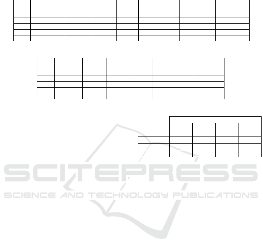
Table 1: Comparison between the two methods.
#inst Flight Dur (min) K
1
(min) #nodes Percentage of V ExecT1 (min) ExecT2 (ms)
1 NCE → DXB 360 0 287 2.5 % 53 2321
2 JFK → NCE 490 198 156 1.3 % 51 1127
3 CDG → SCL 870 245 56 0.49 % 55 696
4 LHR → ATL 565 330 771 6.82 % 51 786
5 FRA → PEK 550 198 416 3.68 % 53 736
6 AMS → IST 195 0 65 0.57 % 57 693
Table 2: Time needed to solve the flight radius problem with two criteria.
#inst Dur (min) K
1
(min) K
2
(usd) #nodes Percentage of V ExecT (ms)
1 360 0 0 1200 10.62 % 3604
2 490 198 17.0 590 5.22 % 1657
3 870 245 42.98 479 4.23 % 1597
4 565 330 96.14 1424 12.60 % 1906
5 550 198 17.0 933 8.25 % 1742
6 195 0 0 477 4.22 % 1554
a measure of central tendency. MCT is ignored for the
cost criterion. Setting K to zero, for example, means
that the subgraph contains all the shortest paths pass-
ing through the arc studied (o, d). On the contrary,
setting K to a high value implies that the subgraph
contains all nodes of the condensed graph. Note that
the MCT is set to 120 minutes. Besides, we generate
100 instances that include for each pair of (OD) gen-
erated randomly, 10 tests with different classes of two
criteria.
Problem with One Criterion. Tests have been run
on existing flights between various airports in terms
of degree. We apply the query for the time criterion
since it takes a lot of time to solve the whole prob-
lem. Table 1 gives the results of testing both methods.
#nodes: the order of output subgraph. Dur: flight du-
ration of the arc studied, the parameter K
1
fixed for
each test, and the percentage of nodes filtered. Ex-
ecT1 presents the running time of the first method
whereas Exect2 is for the second method. The run-
ning time of method based on a query is very impor-
tant. Neo4j Implements bidirectional Dijkstra’s al-
gorithm. So, the algorithm is repeated for each pair
of nodes individually to find the shortest path from
a node to all other nodes. Thus, many computations
are repeated. However, our algorithm used the single-
source shortest path algorithm. So, we are seeking
to return the shortest path tree; that is, the shortest
path from source to all nodes. But the result returned
is a list of paths. That means, in terms of spatial
complexity, the sum of the length of the n paths se-
lected is bound by n
2
in the case of multiple runs of
single-source shortest path algorithms rather than n
paths in the case of three returned with n the num-
ber of nodes in the graph. The time complexity is
O(n × (m + n log n)) as it runs multiple times as the
Table 3: Average run time for various regrets.
Class cost
Class time 0 1 2 3
0 1573.6 1590.4 1657.2 2354.8
1 1783.2 1677.0 1759.4 2246.0
2 1877.8 2007.3 1928.1 2248.0
3 1367.0 2271.5 1484.1 1491.5
order of the graph. In the worst case. The query runs
in 57 minutes whereas, the algorithm takes only 2321
ms. Therefore, the algorithm outperforms the query.
Problem with Two Criteria. Table 2 gives the re-
sult of running the flight radius algorithm with two
criteria. The percentage of supported nodes increases
as we add a second criterion. Even with zero re-
gret, the percentage is at least twice than the percent-
age with 1 criterion. For the instance 1 and 6, the
subgraph contains all shortest paths passing by these
flights: (NCE, DXB) and (AMS,IST) for both criteria
time and cost. In the instance 2, 3, and 4, the regret is
chosen respectively to the quartiles: Q
1
, Q
2
, and Q
3
.
Table 3 gives the average running time as a func-
tion of classes of parameter K
1
and K
2
. The aver-
age running time increases slightly when both value
increase. The algorithm runs in the best case when
the parameter K
1
is set to a value greater than the
third quartile which represents 75 % of flight dura-
tion whereas K
2
is setting to zero. In the worst case,
the algorithm runs twice than in the best case. It is
achieved when we swap both values. It comes back
to the choice of the parameter K
1
since it is computed
in relation with the minimum connection time MCT .
Then, the algorithm is influenced by the second pa-
rameter.
ICORES 2018 - 7th International Conference on Operations Research and Enterprise Systems
310

8 CONCLUSIONS
This work presents the flight radius problem. We
formulated the problem as finding a maximal sub-
graph, in terms of nodes, such that each node sup-
ports a valid path by the regret function. Then, we
presented two methods to solve the problem. Method
using procedures of Neo4j the graph database where
the condensed graph is stored and, the method based
on a new algorithm that relies on Dijkstra algo-
rithm. Test instances are based on the real-world net-
work. The algorithm outperforms the query method
and the choice of the parameter K influences the
running time of the algorithm. Later, we aim to
test the algorithm on benchmark graphs to test the
performance when the topology changes. Also, we
aim to test another shortest path algorithms which is
Bellman-Ford since it takes O(nm) in the worst case
and paths in flight network are characterized by small
length in terms of the number of arcs.
REFERENCES
Ahuja, R. K., Magnanti, T. L., and Orlin, J. B. (1993).
Network flows: theory, algorithms, and applications.
Prentice hall.
Barnhart, C., Belobaba, P., and Odoni, A. R. (2003). Ap-
plications of operations research in the air transport
industry. Transportation science, 37(4):368–391.
Barnhart, C. and Cohn, A. (2004). Airline schedule plan-
ning: Accomplishments and opportunities. Manufac-
turing & service operations management, 6(1):3–22.
Cherkassky, B. V., Goldberg, A. V., and Radzik, T. (1996).
Shortest paths algorithms: Theory and experimental
evaluation. Mathematical programming, 73(2):129–
174.
Hall, R. (2012). Handbook of transportation science, vol-
ume 23. Springer Science & Business Media.
Holzschuher, F. and Peinl, R. (2014). Performance op-
timization for querying social network data. In
EDBT/ICDT Workshops, pages 232–239.
Jacobs, T. L., Garrow, L. A., Lohatepanont, M., Koppel-
man, F. S., Coldren, G. M., and Purnomo, H. (2012).
Airline planning and schedule development. In Quan-
titative Problem Solving Methods in the Airline Indus-
try, pages 35–99. Springer.
Larsson, P. (2008). Analyzing and adapting graph algo-
rithms for large persistent graphs. Master’s thesis.
Neo4j (2017). https://www.neo4j.com.
Pajor, T. (2009). Multi-modal route planning. PhD thesis,
Universitat Karlsruhe (TH) - Institut fr Theoretische
Informatik (ITI).
Rebetanety, A. (2006). Airline schedule planning integrated
flight schedule design and product line design. Uni-
versity Karlsruhe (TH). PhD thesis.
Robinson, I., Webber, J., and Eifrem, E. (2015). Graph
databases: new opportunities for connected data.
”O’Reilly Media, Inc.”.
Solving the Flight Radius Problem
311