
A Lock-free Algorithm for Parallel MCTS
S. Ali Mirsoleimani
1,2
, Jaap van den Herik
1
, Aske Plaat
1
and Jos Vermaseren
2
1
Leiden Centre of Data Science, Leiden University, Niels Bohrweg 1, 2333 CA Leiden, The Netherlands
2
Nikhef Theory Group, Nikhef Science Park 105, 1098 XG Amsterdam, The Netherlands
Keywords:
MCTS, Tree Parallelization, Lock-free Tree, Synchronization Overhead, Memory Ordering.
Abstract:
In this paper, we present a new lock-free tree data structure for parallel Monte Carlo tree search (MCTS) which
removes synchronization overhead and guarantees the consistency of computation. It is based on the use of
atomic operations and the associated memory ordering guarantees. The proposed parallel algorithm scales
very well to higher numbers of cores when compared to the existing methods.
1 INTRODUCTION
In the last decade, there has been much interest in the
MCTS algorithm. The start was by a new, adaptive,
randomized optimization algorithm (Coulom, 2006;
Kocsis and Szepesv´ari, 2006). In fields as diverse
as Artificial Intelligence, Combinatorial Optimiza-
tion, and High Energy Physics, research has shown
that MCTS can find approximate answers without
domain-dependent heuristics (Kocsis and Szepesv´ari,
2006; Kuipers et al., 2013). The strength of the
MCTS algorithm is that it provides answers for any
fixed computational budget with a random amount of
error (Goodfellowet al., 2016). Typically, the amount
of error can be diminished by expanding the com-
putational budget for more running time. In the last
ten years, much effort has been put into the develop-
ment of parallel algorithms for MCTS. The domain
of research contains a broad spectrum of parallel sys-
tems; ranging from small shared-memory multi-core
machines to large distributed-memory clusters. The
goal is to reduce the running time.
One of the approaches for parallelizing MCTS
for shared-memory systems is tree parallelization
(Chaslot et al., 2008a). The method is called so be-
cause a search tree is shared among multiple parallel
threads. Each iteration of the MCTS has four opera-
tions (SELECT, EXPAND, PLAYOUT, and BACKUP).
They are executed on the shared tree simultaneously
(Chaslot et al., 2008b). The MCTS algorithm uses
the tree for storing the states of the domain and guid-
ing the search process. The basic premise of the tree
in MCTS is relatively straight forward: (a) nodes are
added to the tree in the same order as they were ex-
panded and (b) nodes are updated in the tree in the
same order as they were selected. Therefore the fol-
lowing holds, if two parallel threads are performing
the task of adding (EXPAND) or updating (BACKUP)
the same node, there are potentially race conditions.
Thus, one of the main challenges in tree paralleliza-
tion is the prevention of race conditions.
In a parallel program a race condition shows a
non-deterministic behavior that is generally consid-
ered to be a programming error (Williams, 2012).
This behavior occurs when parallel threads perform
operations on the same memory location without
proper synchronization and one of the memory op-
erations is a write. A program with a race condition
may operate correctly sometimes and fail other times.
Therefore, proper synchronizationhelps to coordinate
threads to obtain the desired runtime order and avoid
a race condition.
There are two lock-based methods to create syn-
chronization in tree parallelization: (1) a coarse-
grained lock (Chaslot et al., 2008a), (2) a fine-grained
lock (Chaslot et al., 2008a).
Both methods are straight forward to design and
to implement. However, locks are notoriously bad for
parallel performance, because other threads have to
wait until the lock is released. This is called syn-
chronization overhead. It is shown that the fine-
grained lock has less synchronization overhead than
the coarse-grained lock (Chaslot et al., 2008a). Yet,
even fine-grained locks are often a bottleneck when
many threads try to acquire the same lock. Hence, a
lock-free tree data structure for parallelized MCTS is
desirable and has the potential for maximal concur-
rency. A tree data structure is lock-free when more
than one thread must be able to access its nodes con-
currently. Here, the problem is that the development
of a lock-free tree for parallelized MCTS is shown to
be non-trivial. The difficulty of designing an adequate
Mirsoleimani, S., Herik, J., Plaat, A. and Vermaseren, J.
A Lock-free Algorithm for Parallel MCTS.
DOI: 10.5220/0006653505890598
In Proceedings of the 10th International Conference on Agents and Artificial Intelligence (ICAART 2018) - Volume 2, pages 589-598
ISBN: 978-989-758-275-2
Copyright © 2018 by SCITEPRESS – Science and Technology Publications, Lda. All rights reserved
589

data structure stimulated the researchers in the com-
munity to come up with a spectrum of ideas (Enzen-
berger and M¨uller, 2010; Baudiˇs and Gailly, 2011).
As a case in point, Enzenberger et al. compromised
over the correctness of computation. They accepted
faulty results to have a lock-free search tree (Enzen-
berger and M¨uller, 2010). In Below, we propose
a new lock-free tree data structure without compro-
mises together with the corresponding algorithm that
uses the tree for parallel MCTS.
The remainder of this paper is structured as fol-
lows. Section 2 briefly provides the required back-
ground information. Section 3 discusses related work.
Section 4 presents the proposed lock-free algorithm.
Section 5 shows implementation details. Section 6
gives the experimental setup, and Section 7 provides
the experimental results. Finally, a conclusion is
given in Section 8.
2 BACKGROUND
Below we discuss MCTS in Section 2.1, the UCT al-
gorithm in Section 2.2, and tree parallelization in Sec-
tion 2.3.
2.1 The MCTS Algorithm
The MCTS algorithm iteratively repeats four steps
(also called operations) to construct a search tree un-
til a predefined computational budget (i.e., time or it-
eration constraint) is reached (Chaslot et al., 2008b;
Coulom, 2006). Algorithm 1 shows the general
MCTS algorithm.
At the beginning, the search tree has only a root
(v
0
) which represents the initial state (s
0
) in a domain.
Each node in the search tree resembles a state of
the domain. The edges directed to the child nodes
represent actions leading to succeeding states. Figure
1 illustrates one iteration of the MCTS algorithm on
a search tree that already has nine nodes. The non-
terminal and internal nodes are represented by circles.
Algorithm 1: The generalMCTS algorithm.
1 Function MCTS(s
0
)
2 v
0
:= creat root node with state s
0
;
3 while within search budget do
4 < v
l
,s
l
> := SELECT(v
0
,s
0
);
5 < v
l
,s
l
> := EXPAND(v
l
,s
l
);
6 ∆ := PLAYOUT(v
l
,s
l
);
7 BACKUP(v
l
,∆);
8 end
9 return action a for the best child of v
0
Squares show the terminal nodes.
1. SELECT: A path of nodes inside the search tree is
selected from the root node until a non-terminal
leaf with unvisited children is reached (v
6
). Each
of the nodes inside the path is selected based on a
predefined tree selection policy (see Figure 1a).
2. EXPAND: One of the children (v
9
) of the selected
non-terminal leaf (v
6
) is generated randomly and
added to the tree and also to the selected path (see
Figure 1b).
3. PLAYOUT: From the given state of the newly
added node, a sequence of randomly simulated
actions is performed until a terminal state in the
domain is reached. The terminal state is evaluated
using a utility function to produce a reward value
∆ (see Figure 1c).
4. BACKUP: For each node in the selected path, the
number N(v) of times it has been visited is incre-
mented by 1 and its total reward value Q(v) is up-
dated according to ∆ (Browne et al., 2012). These
values are required by the tree selection policy
(see Figure 1d).
As soon as the computational budget is exhausted, the
best child of the root node is returned (e.g., the one
with the maximum number of visits).
2.2 The UCT Algorithm
This section explains the most common algorithm
in the MCTS family, the Upper Confidence Bounds
for Trees (UCT) algorithm. The UCT algorithm ad-
dresses the exploitation-exploration dilemma in the
selection step of the MCTS algorithm using the UCB1
policy (Kocsis and Szepesv´ari, 2006). A child node j
is selected to maximize:
UCT( j) =
X
j
+ 2C
p
s
2ln(N(v))
N(v
j
)
(1)
Where
X
j
=
Q(v
j
)
N(v
j
)
is an approximation of the
game-theoretic value of node j. Q(v
j
) is the total re-
ward of all playouts that passed through node j, N(v
j
)
is the number of times node j has been visited, N(v)
is the number of times the parent of node j has been
visited, andC
p
≥ 0 is a constant. The left-hand term is
for exploitation and the right-hand term is for explo-
ration (Kocsis and Szepesv´ari, 2006). The decrease or
increase in the amount of exploration can be adjusted
by C
p
in the exploration term. It has profound effect
on the behavior of the algorithm (see Section 7).
ICAART 2018 - 10th International Conference on Agents and Artificial Intelligence
590

v
0
v
1
v
4
v
5
v
8
v
2
v
3
v
6
v
7
(a) SELECT
v
0
v
1
v
4
v
5
v
8
v
2
v
3
v
6
v
9
v
7
(b) EXPAND
v
0
v
1
v
4
v
5
v
8
v
2
v
3
v
6
v
9
∆
v
7
(c) PLAYOUT
v
0
v
1
v
4
v
5
v
8
v
2
v
3
v
6
v
9
v
7
∆
∆
∆
(d) BACKUP
Figure 1: One iteration of MCTS.
2.3 Tree Parallelization
There are three parallelization methods for MCTS
(i.e., root parallelization, leaf parallelization, and tree
parallelization) that belong to two main categories:
(A) parallelization with an ensemble of trees, and (B)
parallelization with a single shared tree.
The root parallelization method belongs to cate-
gory (A). It creates an ensemble of search trees (i.e.,
one for each thread). The trees are independent of
each other. When the search is over, they are merged,
and the action of the best child of the root is selected.
The leaf parallelization and tree parallelization
methods belong to category (B). In the leaf par-
allelization, the parallel threads perform multiple
PLAYOUT operations from a non-terminal leaf node
of the shared tree. These PLAYOUT operations are
independent of each other, and therefore there is no
race condition. In tree parallelization, parallel threads
are potentially able to perform different MCTS opera-
tions on a same node of the shared tree (Chaslot et al.,
2008a). These shared accesses are the source of the
potential race conditions.
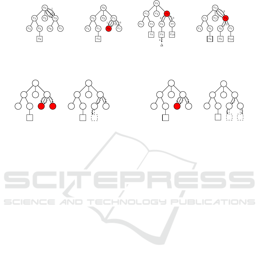
2.4 The Race Conditions
A race condition occurs when concurrent threads per-
form operations on the same memory location with-
out proper synchronization, and one of the memory
operations is a write (McCool et al., 2012). Consider
the example search tree in Figure 2. Three parallel
threads (1, 2, and 3 from v
0
to v
3
) attempt to perform
MCTS operations on the shared search tree. There are
three race condition scenarios.
• Shared Expansion (SE): Figure 2b shows two
threads (1 and 2) concurrently performing EX-
PAND(v
6
). In this SE scenario, synchronization
is required. Obviously, a race condition exists if
two parallel threads intend to add node v
9
to v
6
si-
multaneously. In such an SE race, the child node
should be created and added to its parent only
once.
• Shared Backup (SB): Figure 2c shows two threads
(1 and 3) concurrently performing BACKUP(v
3
).
In the SB scenario, synchronization is required
because there are two data race conditions when
parallel threads update the value of Q(v
3
) and
N(v
3
) simultaneously. There are two dangers: (a)
the value of either Q(v
3
) or N(v
3
) could be cor-
rupted due to concurrently writing them, and (b)
the variable Q(v
3
) and N(v
3
) could be in an incon-
sistent state when the writing of their values does
not happen together at the same time (i.e., the state
of one variable is ahead of the other one).
• Shared Backup and Selection (SBS): Figure 2d
shows thread 2 performing BACKUP(v
3
) and
thread 3 performing SELECT(v
3
). In the SBS sce-
nario, synchronization is required. Otherwise, a
race condition may occur between (i) thread 3
reading the value of Q(v
3
), and (ii) before thread
3 can read the value of N(v
3
), thread 2 updates
the value of Q(v
3
) and N(v
3
). Thus what happens
is that when thread 3 reads the value of N(v
3
),
the variables Q(v
3
) and N(v
3
) are not in the same
state anymore and therefore thread 3 reads an in-
consistent set of values (Q(v
3
) and N(v
3
)).
3 RELATED WORK
In this section, we present the related work for two
categories of synchronization methods for tree paral-
lelization: (1) lock-based methods and (2) lock-free
methods.
3.1 Lock-based Methods
As already mentioned, one of the main challenges in
tree parallelization is to prevent date race conditions
using synchronization. Figure 3 shows the tree paral-
lelization where two threads (1 and 2) simultaneously
perform the EXPAND operation on a node (v
6
) of the
tree. There are two methods to create synchroniza-
tion in this case for tree parallelization: (1) coarse-
grained lock (Chaslot et al., 2008a), (2) fine-grained
lock (Chaslot et al., 2008a):
1. The coarse-grained lock method uses one lock
A Lock-free Algorithm for Parallel MCTS
591
(a) (b)
(c)
(d)
Figure 2: (2a) The initial search tree. The internal and non-terminal leaf nodes are circles. The terminal leaf nodes are squares.
The curly arrows represent threads. (2b) Thread 1 and 2 are expanding node v
6
. (2c) Thread 1 and 2 are updating node v
3
.
(2d) Thread 1 is selecting node v
3
while thread 2 is updating this node.
v
0
v
1
v
4
v
5
v
8
v
2
v
3
v
6
v
7
1
2
3
(a)
v
0
v
1
v
4
v
5
v
8
v
2
v
3
v
6
v
9
v
7
1
2
3
(b)
Figure 3: Tree parallelization with coarse-grained lock.
to protect the entire search tree (Chaslot et al.,
2008a). For example in Figure 3a, both thread
1 and 2 want to expand node v
6
, then thread 1
first acquires a lock; subsequently, it performs the
EXPAND operation and finally releases the lock.
During this process thread 2 also wanting to per-
form the EXPAND operation on node v
6
should
wait for the release of the lock (see Figure 3b).
This method is called coarse-grained because the
access to the tree for performing the EXPAND op-
eration will be given to one and only one thread.
Even if multiple threads want to expand different
nodes inside the tree. For example in Figure 3a,
thread 3 also wants to perform the EXPAND oper-
ation but on node v
7
. However, the lock is already
acquired by thread 1. Therefore, thread 3 should
wait until the lock is released (see Figure 3b).
2. The fine-grained lock method uses one lock for
each node of the tree to protect a smaller part of
the search tree and to allow a greater level of con-
currency in accesses to the search tree (Chaslot
et al., 2008a). For example in Figure 4a, thread
3 also wants to perform the EXPAND operation
but on node v
7
. It can acquire the lock in v
7
and
should not wait (see Figure 3b).
Both lock-based methods use locks to protect
shared data. However, these approaches suffer from
synchronization overhead due to thread contentions
and do not scale well (Chaslot et al., 2008a). A lock-
free method can remove these problems.
v
0
v
1
v
4
v
5
v
8
v
2
v
3
v
6
v
7
1
2
3
(a)
v
0
v
1
v
4
v
5
v
8
v
2
v
3
v
6
v
9
v
7
v
10
1
2
3
(b)
Figure 4: Tree parallelization with fine-grained lock.
3.2 Lock-free Methods
A lock-free implementation exists in the FUEGO
package (Enzenberger and M¨uller, 2010). However,
the method in (Enzenberger and M¨uller, 2010) does
not guarantee the computational consistency of the
multithreaded program with the single-threaded pro-
gram. To address the SE race condition, Enzenberger
et al. assign to each thread an own memory array for
creating nodes (Enzenberger et al., 2010). Only after
the children are fully created and initialized, they are
linked to the parent node. Of course, this causes mem-
ory overhead. What usually happens is the following.
If severalthreads expand the same node, only the chil-
dren created by the last thread will be used in future
simulations. It can also happen that some of the chil-
dren that are lost in this way already received some
updates; these updates will also be lost. It means that
Enzenberger et al. ignore the SB and SBS race condi-
tions. They accept the possible faulty updates and the
inconsistency of parallel computation.
In the PACHI package (Baudiˇs and Gailly, 2011),
the method in (Enzenberger and M¨uller, 2010) is used
for performinglock-free tree updates. Again, it means
that both SB and SBS race conditions are neglected.
However, to allocate children of a given node, PACHI
does not use a per-thread memory pool as FUEGO
does, but uses instead a pre-allocated global node pool
and a single atomic increment instruction updating the
pointer to the next free node. This solves the memory
overhead problem in FUEGO. However, there are still
two other issues with this method: (1) the number of
required nodes should be known in advance, and (2)
ICAART 2018 - 10th International Conference on Agents and Artificial Intelligence
592

the children of a node may not be assigned in consec-
utive memory locations which results in poor spatial
locality (i.e., if a particular memory location is refer-
enced at a particular time, then it is likely that nearby
memory locations will be referenced in the near fu-
ture). The spatial locality is specifically important for
the SELECT operation.
4 OUR PROPOSED LOCK-FREE
TREE DATA STRUCTURE AND
ALGORITHM
Algorithm 2 shows our new lock-free tree data struc-
ture of type Node. The UCT algorithm that uses the
proposed data structure is given in Algorithm 3 (for
the difference, see the end of this section).
Algorithm 2 uses the new multithreading-aware
memory model of the C++11 Standard (Williams,
2012). To avoid the race conditions, the ordering of
memory accesses by the threads has to be enforced
(Williams, 2012). In our lock-free approach, we use
the synchronization properties of the atomic opera-
tions to enforce an ordering between the accesses.
We have used the atomic variants of the built-in types
(i.e., atomic
int and atomic bool); they are lock-free
on all most popular platforms. The standard atomic
types have different member functions such as load(),
store(), exchange(), fetch
add(), and fetch sub(). The
differences are subtle. The member function load()
is a load operation, whereas the store() is a store op-
eration. The exchange() member function is special.
It replaces the stored value in the atomic variable by
a new value and automatically retrieves the original
value. Therefore, we use two memory models for the
memory-ordering option for all operations on atomic
types: (1) sequentially consistent ordering (mem-
ory
order seq cst) and (2) acquire release ordering
(memory
order acquire and memory order release).
The default behavior of all atomic operations pro-
vides for sequentially consistent ordering. This im-
plies that the behavior of a multithreaded program is
consistent with a single threaded program. In the ac-
quire
release ordering model, load() is an acquire op-
eration, store() is a release operation, exchange() or
fetch
add() or fetch sub() are either acquire, release
or both (memory order acq rel).
In Algorithm 2 each node v stores nine different
pieces of data: (1) a the action to be taken, (2) p
the current player at node v, (3) w
n (a 64-bit atomic
integer) that stores both the total simulation reward
Q(v) and the visit count N(v), (4) the list of chil-
dren, (5) the is
parent flag (an atomic boolean) that
Algorithm 2: The new lock-free tree data
structure.
1 type
2 type a : int;
3 type p : int;
4 type w
n : atomic int 64;
5 type children : Node*[];
6 type is
parent := false : atomic bool;
7 type n
nonexpanded children := -1 : atomic int;
8 type is
expandable := false : atomic bool;
9 type is
fully expanded := false : atomic bool;
10 type parent : Node*;
11 Function CREATECHILDREN(actions) : <void>
12 if is parent.exchange(true) is false then
13 j := 0;
14 while actions is not empty do
15 choose a
′
∈ actions;
16 add a new child v
′
with a
′
as its action
and p
′
as its player to the list of
children;
17 j := j+1;
18 end
19 n
nonexpanded children.store(j);
20 is
expandable.store(
21 true,memory
order release);
22 end
23 Function ADDCHILD() : <Node*>
24 index := -1;
25 if is
expandable.load(memory order acquire) is
true then
26 if (index :=
n
nonexpanded children.fetch sub(1)) is 0
then
27 is fully expanded.store(true);
28 end
29 if index < 0 then
30 return current node;
31 else
32 return children[index];
33 end
34 else
35 return current node;
36 end
37 Function ISFULLYEXPANDED() : <bool>
38 return is fully expanded.load();
39 Function GET() : <int,int>
40 w n
′
:= w n.load();
41 w := high 32 bits of w
n
′
;
42 n := low 32 bits of w
n
′
;
43 return < w, n >;
44 Function SET(int ∆)
45 w n
′
:= 0;;
46 high 32 bits of w
n
′
:= ∆;
47 low 32 bits of w
n
′
:= 1;
48 w
n.fetch add(w n
′
);
49 Function UCT(int n) : <float>
50 < w
′
,n
′
> := GET();
51 return
w
′
n
′
+ 2C
p
q
2ln(n)
n
′
52 Node;
A Lock-free Algorithm for Parallel MCTS
593

Algorithm 3: The Lock-free UCT algo-
rithm.
1 Function UCTSEARCH(Node* v
0
, State s
0
, budget)
2 while within search budget do
3 < v
l
,s
l
> := SELECT(v
0
,s
0
);
4 < v
l
,s
l
> := EXPAND(v
l
,s
l
);
5 ∆ := PLAYOUT(v
l
,s
l
);
6 BACKUP(v
l
,∆);
7 end
8 Function SELECT(Node* v, s) : <Node*,State>
9 while v.ISFULLYEXPANDED() do
10 < w, n > := v.GET();
11 v
l
:= argmax
v
j
∈children of v
v
j
.UCT(n);
12 s := v.p takes action v
l
.a from state s;
13 v := v
l
;
14 end
15 return < v, s >;
16 Function EXPAND(Node* v,State s) : <Node*,State>
17 if s is non-terminal then
18 actions := set of untried actions from state s;
19 v.CREATECHILDREN(actions);
20 v
′
:= v.ADDCHILD();
21 if v
′
is not v then
22 v := v
′
;
23 s := v.p takes action v.a from state s;
24 end
25 end
26 return < v, s >;
27 Function PLAYOUT(State s)
28 while s is non-terminal do
29 choose a ∈ set of untried actions from state s
uniformly at random;
30 s := the current player p takes action a from state s;
31 end
32 ∆(p) := reward for state s for each player p;
33 return ∆
34 Function BACKUP(Node* v,∆) : void
35 while v is not null do
36 v.SET(∆(v.p));
37 v := v.parent;
38 end
shows whether the list of children is already created,
(6) n
nonexpanded children the number of children
that are not expanded yet, (7) the is expandable flag
(an atomic boolean) that shows whether v is ready
to be expanded, (8) the is
fully expanded flag (an
atomic boolean) that shows whether all children of v
are already expanded and (9) parent that points to the
parent of v. By using (a) the atomic variables, (b)
the atomic operations, and (c) the associated memory
models, we can solve all the three above cases of race
conditions (SE, SB, and SBS).
• SE: To solve the SE race condition, the EXPAND
operation in Algorithm 3 consists of two separate
sub-operations: (A) the CREATECHILDREN op-
eration and (B) the ADDCHILD operation. The
first operation has four key steps (A-1, A-2, A-
3, A-4) which are given in Algorithm 2. (A-1):
Exchanging the value of is
parent from false to
true prevents the other threads to create the list
of children (Line 12). Thus, the problem that the
list of children is created by two threads at the
same time is solved. (A-2): Creating the list of
children (Line 14-18). (A-3): Set the value of
n
nonexpanded children to counter j (Line 19),
(A-4): Set the value of is expandable to true
(Line 20). After a node successfully has become
a parent, one of the non-expanded children in its
list of children can be added using the ADDCHILD
operation. The ADDCHILD operation in Algo-
rithm 2 has three key steps (B-1, B-2, B-3). (B-1):
Read the value of is
expandable (Line 24), if it is
true, try to expand a new child (Line 25-32). Oth-
erwise, return the current node (Line 34). (B-2):
The value of index is calculated (Line 25), if it
is zero, then node v is fully expanded (Line 26).
(B-3): index shows the next child to be expanded
(Line 31), if index becomes negative, the current
node is returned (Line 29).
• SB: To solve the SB race condition, Algorithm 2
uses a single 64-bit atomic integer w
n for storing
both variables Q(v) and N(v). The value of Q(v)
is stored in the high 32 bits of w
n, while the value
of N(v) is stored in low 32 bits. This compression
technique preserves the correct state of the vari-
ables Q(v) and N(v) in all threads because they
should always be written together using a SET op-
eration. Therefore, we have no faulty updates and
guarantee consistency of computation.
• SBS: To solve the SBS race condition, Algorithm
3 always reads w
n variable by a GET operation
in the SELECT operation. The GET operation al-
ways reads the value of Q(v) and N(v) together.
If a BACKUP operation wants to update the w
n
variable in the same time, it happens through a
SET operation which writes the value of Q(N) and
N(v) together. Therefore, the value of Q(v) and
N(v) are always correct, in the same state, and
consistency of computation is guaranteed.
In Algorithm 3, each node v is also associated with
a state s. The state s is recalculated as the SELECT
and EXPAND steps descend the tree. The term ∆(p)
denotes the reward after simulation for each player.
ICAART 2018 - 10th International Conference on Agents and Artificial Intelligence
594

Algorithm 4: The pseudo-code of GSCPM
algorithm.
1 Function GSCPM(State s
0
,nPlayouts,nTasks)
2 v
0
:= create a shared root node with state s
0
;
3 grain
size := nPlayouts/nTasks;
4 t:= 1;
5 for t ≤ nTasks do
6 s
t
:=s
0
;
7 fork UCTSEARCH(v
0
,s
t
,grain
size) as task t;
8 t:=t+1;
9 end
10 wait for all tasks to be completed;
11 return action a of best child of v
0
;
5 IMPLEMENTATION
We have implemented the proposed lock-free data
structure and algorithm in the ParallelUCT package
(Mirsoleimani et al., 2015). The implementation is
available online as part of the package. The Paral-
lelUCT package is an open source tool for paralleliza-
tion of the UCT algorithm.
1
It uses task-level paral-
lelism to implement different parallelization methods
for MCTS. We have used an algorithm called grain-
sized control parallel MCTS (GSCPM) to implement
and measure the performance of the proposed lock-
free UCT algorithm. The pseudo-code for GSCPM is
given in Algorithm 4. The GSCPM is implemented
by multiple methods from different parallel program-
ming libraries such as C++11 STL, thread pool (TP-
FIFO), TBB (task
group) (Reinders, 2007), and Cilk
Plus (cilk for and cilk spwan) (Robison, 2013) in the
ParallelUCT package. More details about each of
these methods can be found in (Mirsoleimani et al.,
2015).
6 EXPERIMENTAL SETUP
Section 6.1 discusses our case study, Section 6.2 ex-
plains the performance metrics, and Section 6.3 pro-
vides the details of hardware.
6.1 The Game of Hex
The performance of the lock-free algorithm is mea-
sured by using the game of Hex. Hex is a board game
with a diamond-shaped board of hexagonal cells (Ar-
neson et al., 2010). The game is usually played on a
board of size 11 on a side, for a total of 121 hexagons,
as illustrated in Figure 5 (Weisstein, 2017). Each
player is represented by a color (Black or White).
1
https://github.com/mirsoleimani/paralleluct/
Figure 5: A sample board for the game of Hex
Players take turns by placing a stone of their color
on a cell on the board. The goal for each player is
to create a connected chain of stones between the op-
posing sides of the board marked by their colors. The
first player to complete this path wins the game. The
game cannot end in a draw since no path can be com-
pletely blocked except by a complete path of the op-
posite color. Since the first player to move in Hex
has a distinct advantage, the swap rule is generally
implemented for fairness. This rule allows the sec-
ond player to choose whether to switch positions with
the first player after the first player has made the first
move.
In our implementation of Hex, a disjoint-set data
structure is used to determine the connected stones.
Using this data structure the evaluation of the board
position to find the player who won the game becomes
very efficient (Galil and Italiano, 1991).
6.2 Performance Metrics
One important metric related to performance and par-
allelism is speedup. Speedup compares the time for
solving the identical computational problem on one
worker versus that on P workers:
speedup =
T
1
T
P
. (2)
Where T
1
is the time of the program with one
worker and T
p
is the time of the program with P work-
ers. In our results we report the scalability of our par-
allelization as strong scalability which means that the
problem size remains fixed as P varies. The problem
size is the number of playouts (i.e., the search budget)
and the P is the number of tasks. In the literature this
form of speedup is called playout-speedup (Chaslot
et al., 2008a).
The second important metric in two-player games,
such as Hex, is the percentage of win for method a
versus method b:
win(%) =
W
a
W
a
+W
b
∗ 100. (3)
Where W
a
is the number of wins for method a and
W
b
is the number of wins for method b. If there is a
draw, it will be counted as a win for both players. In
A Lock-free Algorithm for Parallel MCTS
595
Hex, there is always a winner. We note that we have
used the swap rule. Each method played half of the
games as Black and the other half as White.
6.3 Hardware
Our experiments were performed on a dual socket In-
tel machine with 2 Intel Xeon E5-2596v2 CPUs run-
ning at 2.4 GHz. Each CPU has 12 cores, 24 hyper-
threads, and 30 MB L3 cache. Each physical core has
256KB L2 cache. The peak TurboBoost frequency is
3.2 GHz. The machine has 192GB physical memory.
We compiled the code using the Intel C++ compiler
with a -O3 flag.
7 EXPERIMENTAL RESULTS
In Section 7.1, the scalability is studied and the
achieved playout-speedup is reported. The effect of
differences in values of C
p
parameters on the speedup
of the parallel algorithm is measured in Section 7.2.
The performance of the proposed lock-free algorithm
for tree parallelization when playing against root par-
allelization is reported in Section 7.3.
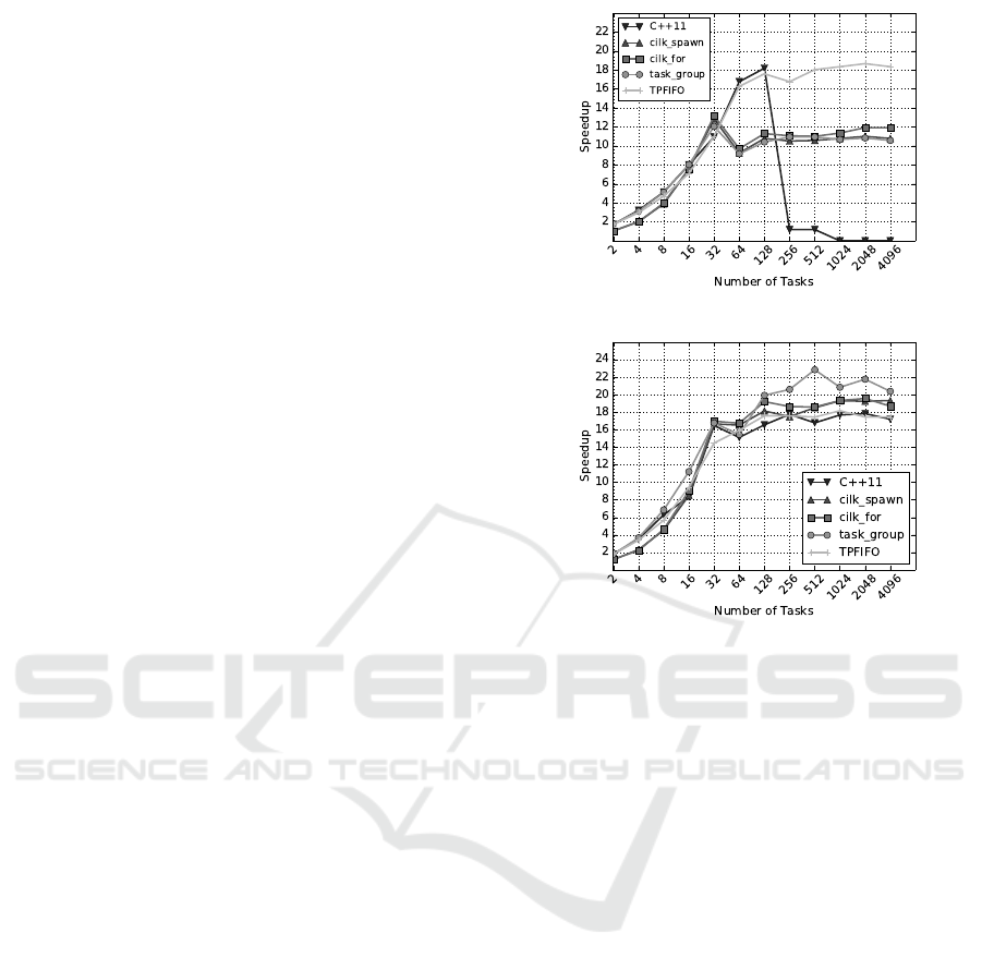
7.1 Playout-speedup
As mentioned before, we are interested in strong
scalability. Therefore, the search budget is fixed to
1,048,576 playouts as the number of tasks are increas-
ing. Figure 6 shows the scalability of the algorithm
for different parallel programming libraries when the
first move on the empty board is made. Each data
point is the average of 21 games. Figure 6a illustrates
the scalability when a coarse-grained lock is used
(The graph is taken from (Mirsoleimani et al., 2015))
and Figure 6b demonstrates the scalability when the
proposed lock-free method is used. There are three
main improvements when the lock-free tree is used:
(1) the maximum speedup increased from 18 to 23.
(2) the scalability of all methods is improved(It shows
the notoriously bad effect of locks on the scalability
for Cilk Plus, TBB, and C++11). (3) 32 tasks are suf-
ficient to reach near 17 times speedup, while for the
lock-based method at least 64 tasks are required.
7.2 The Effect of C
p
on Playout-speedup
Table 1 shows the execution time of the sequential
UCT algorithm for three different C
p
values. It is
observed that the execution time is decreasing as the
value of C
p
is increasing. There is an obvious ex-
planation for this behavior. When the algorithm uses
(a)
(b)
Figure 6: The scalability of tree parallelization for different
parallel programming libraries when C
p
= 1. 6a Coarse-
grained lock. 6b Lock-free.
high exploitation (i.e., low value for C
p
), it constructs
a search tree that is deeper and more asymmetric. In
Figure 7b, the depth of the tree is 56 when the num-
ber of tasks is 1 and C
p
= 0. When the shape of the
tree is more asymmetric, each iteration of the algo-
rithm must traverse a deeper path of nodes inside the
tree using the SELECT operation until it can perform
a PLAYOUT operation. The SELECT operation con-
sist of a while loop which for a tree with the depth of
56 has to perform 56 iterations in the worst case (see
Algorithm 3). The BACKUP operation also consists
of a while loop which for a deeper tree has more iter-
ations. These two operations are also memory inten-
sive ones (i.e., accessing the nodes of the tree which
reside in memory). The results are that the execution
time of the sequential algorithm becomes higher for
high exploitation. Increasing the value of C
p
means
more exploration and thus a more symmetric tree with
a lower depth. In Figure 7b, the depth of the tree is 5
when the number of tasks is 1 and C
p
= 1. In this
case, the while loop in the SELECT operation has to
perform only 5 iterations in the worst case.
We have measured the scalability of the proposed
lock-free algorithm for different C
p
values (see Fig-
ICAART 2018 - 10th International Conference on Agents and Artificial Intelligence
596
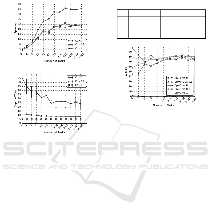
(a)
(b)
Figure 7: 7a The scalability of the algorithm for different
C
p
values. 7b The changes in the depth of tree when the
number of tasks are increasing.
ure 7a). The sequential time for each C
p
in Table 1
is used as the baseline. The maximum speedup for
C
p
= 0 is around 34. It is much higher than 23 times,
the speedup when C
p
= 1. There is a possible expla-
nation for the higher speedup. The parallel algorithm
may be more efficient than the equivalent serial al-
gorithm, since the parallel algorithm may be able to
avoid work that in every serialization would be forced
to be performed (McCool et al., 2012). For exam-
ple, Figure 7b shows the changes in the depth of the
constructed tree with regards to the number of tasks
for three different C
p
. Increasing the number of tasks
reduces the depth of the tree from 56, when the se-
rial execution is exploitative (i.e., C
p
= 0), to around
25. It means that, in parallel execution (a) threads ex-
plore different branches of the tree and (b) the tree
is more symmetric compared to the serial execution.
Hence, the number of iterations in both SELECT and
BACKUP operations reduces in parallel execution and
therefore causes a higher speedup. When the serial
execution has high exploration (i.e., C
p
= 1), increas-
ing the number of tasks does not change the depth of
the tree.
Table 1: Sequential execution time in seconds.
C
p
Time (s) Depth of Tree (Avg.)
0 59.97± 10.93 56.66± 12.16
0.1 26.66± 0.81 11.52± 0.98
1 20.7± 0.3 5
Figure 8: The playing results for lock-free tree paralleliza-
tion versus root parallelization. The first value for C
p
is
used for tree parallelization and the second value is used for
root parallelization.
7.3 Playing vs. Root Parallelization
In this section, the result of playing Hex between
the proposed lock-free tree parallelization against root
parallelization is presented. Root parallelization is
also a parallelization method that does not use locks
because it uses an ensemble of independent search
trees. Therefore, it is interesting to see the perfor-
mance of the proposed lock-free algorithm versus root
parallelization. Figure 8 reports the percentage of
win for lock-free tree parallelization for five differ-
ent combinations of C
p
. Both methods use a same
number of tasks. For each data point, 100 games are
played.
When C
p
= 0 for both algorithms, tree paralleliza-
tion cannot win against root parallelization. It shows
that the high speedup for C
p
= 0 (see Figure 7a) is
not useful. However, when the value of C
p
is selected
to be more exploratory, the lock-free tree paralleliza-
tion is superior to root parallelization, specifically for
a higher number of tasks.
8 CONCLUSION
Monte Carlo Tree Search (MCTS) is a randomized
algorithm that is successful in a wide range of opti-
mization problems. The main loop in MCTS consists
of individual iterations for constructing a search tree,
A Lock-free Algorithm for Parallel MCTS
597

suggesting that the algorithm is well suited for paral-
lelization. The existing tree parallelization for MCTS
uses a shared search tree and runs the iterations in par-
allel. However, the shared search tree has potential
race conditions. In this paper, we have presented a
new lock-free algorithm that has no race conditions. It
showed better scalability and playout-speedup when
compared to other synchronization methods. Cur-
rently, we have used the default sequential consis-
tency memory ordering for all atomic operations be-
cause that is the most convenient way to explain the
intricacies. For future work, we will look at reduc-
ing a selected set of the ordering constraints to the
relaxed-memory ordering.
ACKNOWLEDGEMENTS
This work is supported in part by the ERC Advanced
Grant no. 320651, “HEPGAME.”
REFERENCES
Arneson, B., Hayward, R. B., and Henderson, P. (2010).
Monte Carlo Tree Search in Hex. IEEE Transac-
tions on Computational Intelligence and AI in Games,
2(4):251–258.
Baudiˇs, P. and Gailly, J.-l. (2011). Pachi: State of the Art
Open Source Go Program. In Advances in Computer
Games 13, pages 24–38.
Browne, C. B., Powley, E., Whitehouse, D., Lucas, S. M.,
Cowling, P. I., Rohlfshagen, P., Tavener, S., Perez, D.,
Samothrakis, S., and Colton, S. (2012). A Survey of
Monte Carlo Tree Search Methods. Computational
Intelligence and AI in Games, IEEE Transactions on,
4(1):1–43.
Chaslot, G., Winands, M., and van den Herik, J. (2008a).
Parallel Monte-Carlo Tree Search. In the 6th Interna-
tioal Conference on Computers and Games, volume
5131, pages 60–71. Springer Berlin Heidelberg.
Chaslot, G. M. J. B., Winands, M. H. M., van den Herik, J.,
Uiterwijk, J. W. H. M., and Bouzy, B. (2008b). Pro-
gressive strategies for Monte-Carlo tree search. New
Mathematics and Natural Computation, 4(03):343–
357.
Coulom, R. (2006). Efficient Selectivity and Backup Op-
erators in Monte-Carlo Tree Search. In Proceed-
ings of the 5th International Conference on Comput-
ers and Games, volume 4630 of CG’06, pages 72–83.
Springer-Verlag.
Enzenberger, M. and M¨uller, M. (2010). A lock-free mul-
tithreaded Monte-Carlo tree search algorithm. Ad-
vances in Computer Games, 6048:14–20.
Enzenberger, M., Muller, M., Arneson, B., and Segal, R.
(2010). FuegoAn Open-Source Framework for Board
Games and Go Engine Based on Monte Carlo Tree
Search. IEEE Transactions on Computational Intelli-
gence and AI in Games, 2(4):259–270.
Galil, Z. and Italiano, G. F. (1991). Data Structures and
Algorithms for Disjoint Set Union Problems. ACM
Comput. Surv., 23(3):319–344.
Goodfellow, I., Bengio, Y., and Courville, A. (2016). Deep
Learning. Adaptive Computation and Machine Learn-
ing Series. MIT Press.
Kocsis, L. and Szepesv´ari, C. (2006). Bandit based Monte-
Carlo Planning Levente. In F¨urnkranz, J., Scheffer, T.,
and Spiliopoulou, M., editors, ECML’06 Proceedings
of the 17th European conference on Machine Learn-
ing, volume 4212 of Lecture Notes in Computer Sci-
ence, pages 282–293. Springer Berlin Heidelberg.
Kuipers, J., Plaat, A., Vermaseren, J., and van den Herik, J.
(2013). Improving Multivariate Horner Schemes with
Monte Carlo Tree Search. Computer Physics Commu-
nications, 184(11):2391–2395.
McCool, M., Reinders, J., and Robison, A. (2012). Struc-
tured Parallel Programming: Patterns for Efficient
Computation. Elsevier.
Mirsoleimani, S. A., Plaat, A., van den Herik, J., and Ver-
maseren, J. (2015). Parallel Monte Carlo Tree Search
from Multi-core to Many-core Processors. In ISPA
2015 : The 13th IEEE International Symposium on
Parallel and Distributed Processing with Applications
(ISPA), pages 77–83, Helsinki.
Reinders, J. (2007). Intel threading building blocks: out-
fitting C++ for multi-core processor parallelism. ”
O’Reilly Media, Inc.”.
Robison, A. D. (2013). Composable Parallel Patterns with
Intel Cilk Plus. Computing in Science & Engineering,
15(2):66–71.
Weisstein, E. W. (2017). Game of hex. From MathWorld—
A Wolfram Web Resource.
Williams, A. (2012). C++ Concurrency in Action: Prac-
tical Multithreading. Manning Pubs Co Series. Man-
ning.
ICAART 2018 - 10th International Conference on Agents and Artificial Intelligence
598
