Denoising Monte Carlo Renderings based on a Robust High-order
Function
Yu Liu
1,2
, Changwen Zheng
1
and Hongliang Yuan
1,2
1
Institute of Software, Chinese Academy of Sciences, Beijing, China
2
University of Chinese Academy of Sciences, Beijing, China
Keywords:
Adaptive Rendering, Image Space Reconstruction, Guided Image Filter, Mean Squared Error.
Abstract:
Image space rendering methods are efficient at removing Monte Carlo noise. However, a major challenge is
optimizing the bandwidth to denoise images while preserving their fine details. In this paper, a high-order
function is proposed to leverage the correlation between features and pixel colors. We consider feature buffers
to fit data while computing regression weights using pixel colors. A collaborative prefiltering framework is
first proposed to denoise features. The input pixel colors are then denoised using a guided image filter that
maintains fine details in the output by constructing a guidance image using features. The optimal bandwidth
is selected through an iterative error estimation process performed at multiple pixels to smooth the details.
Finally, we adaptively select center pixels to build our regression models and vary the window size to reduce
computational overhead. Experimental results showed that the new approach outperforms competing methods
in terms of the quality of the visual image and the numerical error incurred.
1 INTRODUCTION
Monte Carlo (MC) ray tracing (Kajiya, 1986) is a
powerful technique to synthesize photo-realistic im-
ages. It computes a complex multidimensional in-
tegral at each pixel to calculate the scene function.
However, a large number of samples is often required
to produce a visually pleasing result. To solve this
problem, a number of adaptive rendering methods
have been proposed (Li et al., 2012; Rousselle et al.,
2013; Rousselle et al., 2011). The crucial step is the
error analysis of a noisy image produced from few
samples. Based on the analysis, appropriate parame-
ters are selected at each pixel to enable a satisfactory
trade-off between bias and variance, which amounts
to minimizing the mean squared error (rMSE).
Adaptive rendering methods can be classified into
multidimensional and image space techniques. Mul-
tidimensional methods (Hachisuka et al., 2008) are
used in a high-dimensional space where each coor-
dinate corresponds to a random parameter. However,
they are restricted by the curse of dimensionality, and
can only support a limited set of distributed effects.
Image space methods have recently received attention
owing to their simplicity and efficiency. Moreover,
many feature buffers have been used to direct error
analysis. At an abstract level, we can categorize im-
age space methods into two categories: low-order and
high-order functions.
Low-order functions model the neighborhood of a
pixel as a constant regression to perform bandwidth
optimization, whereas high-order ones measure the
varying importance of different features and predict
values both for the center pixel and its neighboring
pixels. For example, weighted local regression is in-
troduced to reconstruct pixels (Moon et al., 2014).
However, these methods are prone to overfitting to the
noisy input (Bako et al., 2017).
In this paper, we determine the order of our re-
gression function to be one since it presents a nice
trade-off between performance and complexity. The
noise in features is first removed using a collaborative
prefiltering framework. We then leverage the corre-
lation between features and pixel colors to robustly
construct a high-order model and regression weights.
In particular, the input pixel colors are denoised using
a guided image filter (GIF) (He et al., 2010), which al-
leviates the problem of overfitting to noisy input. We
then iteratively estimate the reconstruction error in a
patch-wise manner to denoise multiple pixels. Finally
we adaptively select center pixels to build our high-
order models. Experimental results showed that our
method is superior to competing methods on a wide
variety of rendering effects.
288
Liu, Y., Zheng, C. and Yuan, H.
Denoising Monte Carlo Renderings based on a Robust High-order Function.
DOI: 10.5220/0006650602880294
In Proceedings of the 13th International Joint Conference on Computer Vision, Imaging and Computer Graphics Theory and Applications (VISIGRAPP 2018) - Volume 1: GRAPP, pages
288-294
ISBN: 978-989-758-287-5
Copyright © 2018 by SCITEPRESS – Science and Technology Publications, Lda. All rights reserved

2 RELATED WORK
Multidimensional Space Rendering. Hachisuka et
al. (Hachisuka et al., 2008) proposed an anisotropic
reconstruction using a structure tensor. Durand et al.
(Durand et al., 2005) described how the frequency
content of radiance was influenced by varying phe-
nomena, and many algorithms are proposed to im-
prove the image quality of specific effects (Soler et al.,
2009; Egan et al., 2009; Egan et al., 2011). Recently,
Lehtinen et al. (Lehtinen et al., 2011) used depth and
motion information to simulate a wide variety of ef-
fects. Belcoulr et al. (Belcour et al., 2013) performed
a five-dimensional frequency analysis to simulate mo-
tion blur and depth of field. These methods typically
produce impressive results for specific rendering ef-
fects. However, they tend to show poor effectiveness
as the dimensions increased.
Low-order Functions. Low-order methods often
use techniques developed for image processing.
Kalantari et al. (Kalantari and Sen, 2013) proposed to
enable any spatial image filters to denoise MC render-
ings. Many methods selected the optimal bandwidth
using varying error metrics. Li et al. (Li et al., 2012)
used Steins unbiased risk (SURE) to select suitable
parameter. However, SURE estimates can be inaccu-
rate at low sampling rates. Sen et al. (Sen and Darabi,
2012) reduced the importance of samples affected by
noise. Moon et al. (Moon et al., 2013) computed
a virtual flash image to determine the homogeneous
pixels. Delbracio et al. (Delbracio et al., 2014) com-
puted a ray histogram to recognize similar pixels. Re-
cently, Liu et al.(Liu et al., 2017) considered the So-
bel operator to compute a gradient image to prefilter
features.
High-order Functions. High-order functions
mainly measured the varying importance of different
features. Moon et al. (Moon et al., 2014) used a
first-order function to predict center pixels. They
also estimated the optimal function order (Moon
et al., 2016). In addition, a suitable window size is
also computed (Moon et al., 2015) to remove noise.
Kalantari et al. (Kalantari et al., 2015) proposed to
use supervised learning to predict optimal parame-
ters. Recently, Bako et al. (Bako et al., 2017) further
used a convolutional neural network (CNN) to enable
a more complex kernel. Chaitanya et al. (Chaitanya
et al., 2017) introduced a machine learning approach
with low sampling budgets. Readers are encouraged
to read Zwicker et al. work (Zwicker et al., 2015).
3 PROPOSED METHOD
3.1 First-order Regression Function
We define our first-order function as an extension of
zero-order functions:
[y
i
,∇y
i
] = arg min
y
i
,∇y
i
∑
j∈N
i
(y
j
− y
i
− ∇y
i
(x
j
− x
i
))
2
w(i, j)
(1)
where y
i
and ∇y
i
denote the filtered value and the es-
timated gradient at the center pixel i, respectively. N
i
is the reconstruction window. x
i
is a feature vector
used to fit data, and we consider D = 9 dimensional
features: pixel coordinates (2D), depth (1D), normal
(3D), and albedo (3D). w(i, j) is a weight term be-
tween i and j.
As described in a past study (Moon et al., 2015),
a normal equation for the solution is as follows:
y = X(X
T
WX)
−1
X
T
WY (2)
where X is an n ×(D + 1) design matrix the j
th
row of
which is [1, (x
j
−x
i
)
T
], and Y = [y
1
,...y
n
] are the input
colors. W is an n × n diagonal matrix the j
th
element
of which is w(i, j).
y corresponds to all reconstructed
pixel values in N
i
. Eq. (2) enables our model to
predict n pixels in N
i
through one reconstruction step.
3.2 Collaborative Feature Prefiltering
To handle specific effects, the noise in the features
should be removed for computing X. Rousselle
et al. (Rousselle et al., 2013) and Liu et al. (Liu
et al., 2017) proposed denoising features using
image filters, which tend to blur fine details in the
focused or motionless areas. Truncated Singular
Value Decomposition (TSVD) was also used to reject
noisy features. However, it might underestimate local
dimensions and lead to blurred details.
Here, we propose a collaborative process to
denoise features. The input features are first denoised
with a joint-NL-means filter to remove low-frequency
noise and maintain fine feature details. However, it
may leave untreated substantial noise in areas with
complex geometries. We further filter the output of
the joint-NL-means filter using a GIF, which helps re-
move residual noise. As a result, our joint-NL-means
kernel and the GIF form a collaborative framework.
First, we define the joint-NL-means kernel as:
w
jnl
(i, j) = exp
−ki − jk
2
2σ
2
s
exp
−kP
i
− P
j
k
2
2σ
2
r
D−2
∏
m=1
exp
−k f
i,m
− f
j,m
k
2
2σ
2
m
(3)
Denoising Monte Carlo Renderings based on a Robust High-order Function
289

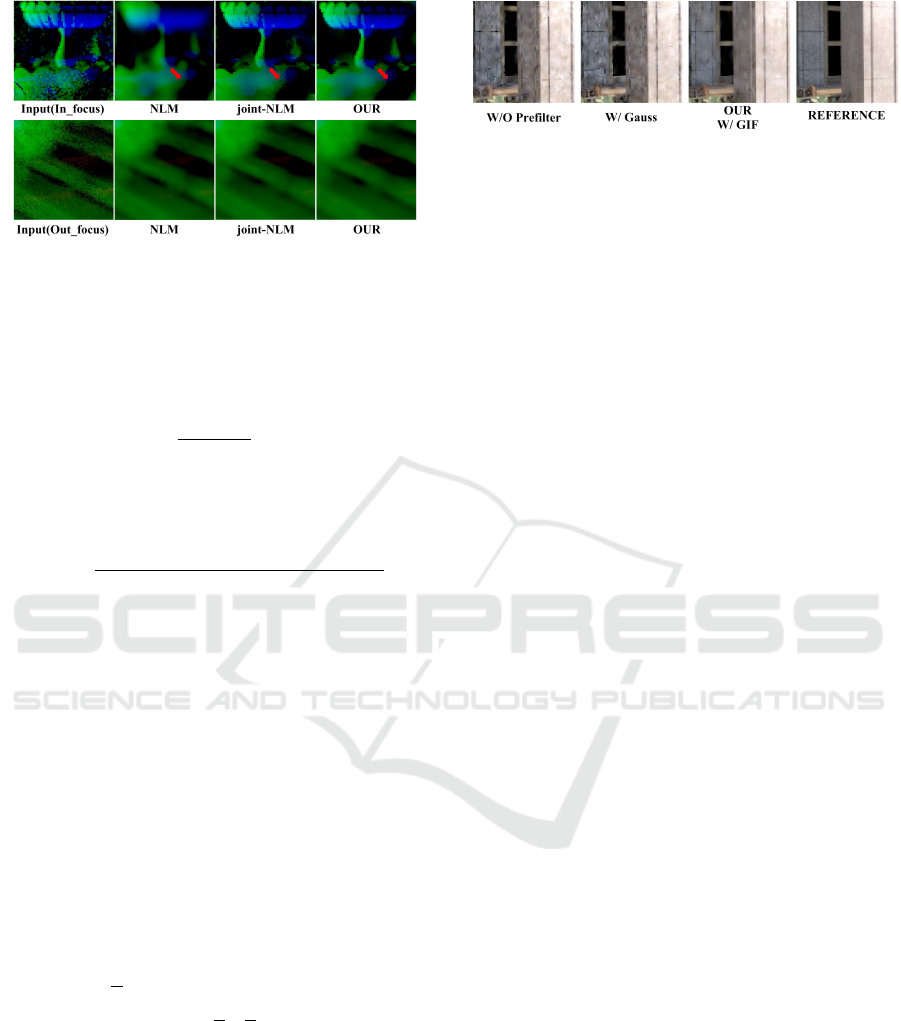
Figure 1: Feature prefiltering in a normal image.
where f
i,m
denote the value of the m
th
feature type
at pixel i. σ
2
s
, σ
2
r
, and σ
2
m
are the variances in the
spatial, the range-related, and the m
th
feature terms,
respectively. kP
i
− P
j
k denotes the patch-based range
P
0
with radius r:
kP
i
−P
j
k
2
= max(0,
1
(2r + 1)
2
∑
l∈P
0
d(i+l, j +l)) (4)
We follow the metric proposed by Rousselle et al.
(Rousselle et al., 2013) to compute the per-pixel range
distance:
d(i, j) =
ky
i
− y
j
k
2
− (var
i
+ min(var
i
,var
j
))
ε + k
2
(var
i
+ var
j
)
(5)
where var
i
is the variance of pixel i, and k is the pa-
rameter used to adjust the strength of the filter.
To this end, we define the NL-means filter as:
b
Y = NLM(Y,k,UF). The input Y is filtered using an
NL-means filter with parameters k, and UF denotes
whether we use the features to form a joint kernel.
Then, the GIF kernel is defined as follows:
b
Y
j
= a
i
I
j
+ b
i
,∀ j ∈ N
i
(6)
where a
i
and b
i
are constant coefficients in N
i
. We
set the regularization parameter to 0.001 to prevent a
j
from becoming too large. Thus a
i
and b
i
can be solved
by using linear regression (He et al., 2010). We sum-
marize the GIF as:
b
Y = GUID(Y,I), where the input
Y is filtered using I as a guidance image.
Given the joint-NL-means and GIF kernels, we fil-
ter the m
th
input feature as follows:
f
m
= NLM( f
m
,0.25,true)
b
f
m
= GUID( f
m
, f
m
)
(7)
where f
m
and
b
f
m
are the input and the output of the
m
th
feature type, respectively. We set σ
s
= 2, σ
r
= 1,
and σ
m
= {0.8,0.25,0.6} for the normal, albedo, and
depth, respectively. Note that each feature channel is
filtered independently.
Fig.1 shows the result of our collaborative pre-
filtering. Note the areas denoted by red arrows. It
is clear that our method can remove the noise while
preserving fine feature details in focused areas.
Figure 2: Denoising color input with a GIF. Our method
uses features to construct a guidance image, which forces
our results to retain fine details while removing initial noise.
3.3 Computing Regression Weight
Using features to compute regression weights can sig-
nificantly improve the quality of zero-order functions.
However, these features can be detrimental to first-
order models. For example, WLR does not con-
sider the color buffer and it produces suboptimal re-
sults when the features fail to recognize scene struc-
tures. Here, we use only pixel colors to compute
the regression weights through an NL-means kernel.
Our regression weights and first-order model are con-
sequently complementary: the feature-based model
recognizes high-frequency scene details whereas the
color-based regression weights preserve elements that
are not captured by the features. Another advantage
of this method is that there is only one parameter k to
set for bandwidth optimization.
Since the input colors are very noisy at low sam-
pling rates, inaccurate results are hence produced be-
cause the high-order functions are prone to overfitting
to noisy color inputs. Here, we denoise the input pixel
colors with a GIF, which forces the filtered result to
have similar edge characteristics to the guidance im-
age. In this case, the features can be selected as the
guidance image as they represent most scene struc-
tures. The input pixel colors y are thus prefiltered:
M
m
= GUID(y,
b
f
m
)
M =
D−2
∑
m=1
M
m
/(D − 2)
(8)
where M
m
is filtered independently using each feature
channel
b
f
m
as a guidance image. Since D− 2 = 7 fea-
ture channels are considered in this paper, M is com-
puted as the average of M
m
. After denoising the ini-
tial pixel colors, the regression weight is computed
as: w(i, j) = NLM(M, k
opt
, f alse). k
opt
is the optimal
bandwidth computed with our iterative error estima-
tion explained in the next section.
Figure 2 shows the results of prefiltering the color
input. After prefiltering with a Gaussian filter (Li
et al., 2012), however, a lot of noise remains. Our
method, owing to the guidance images, produces
smoother details.
GRAPP 2018 - International Conference on Computer Graphics Theory and Applications
290

3.4 Bandwidth Optimization
To minimize the rMSE, a block-based manner is em-
ployed to define our reconstruction error:
k
opt
= argmin
k
∑
j∈N
i
w(i, j)(y
j
− ϕ
j
)
2
(9)
where y
j
and ϕ
j
denote the reconstructed value and
the ground truth at pixel j, respectively. w(i, j) is
the weight between pixel i and j using a candidate
bandwidth k. Eq. (9) cannot be directly computed,
since ϕ
j
can only be obtained with a large number
of samples. Here, we decompose the per-pixel error
err
j,k
= (y
j
−ϕ
j
)
2
of using candidate parameter k into
squared bias bias
2
( j, k) and variance Var(j, k) terms:
k
opt
= argmin
k
∑
j∈N
i
w(i, j)err
j,k
= argmin
k
∑
j∈N
i
w(i, j)(bias
2
( j, k) + Var(j,k))
(10)
To solve Eq. (10), an iterative process is pro-
posed here. In the t
th
iteration, as described in a pre-
vious study (Moon et al., 2016), the bias and vari-
ance terms can be computed using a hat matrix H
(H = X(X
T
WX)
−1
X
T
W):
bias
t
( j, k) =
s=n
∑
s=1
H
j,s
y
s,t−1
− y
j,t−1
Var
t
(j,k) =
s=n
∑
s=1
(H
j,s
)
2
Var
t−1
(s,k)
(11)
where bias
t
( j, k) and Var
t
(j,k) denote the bias and
variance in the t
th
iteration at pixel j, respectively.
H
j,s
is the j
th
row and s
th
column of H. y
s,t−1
is
the output of pixel j in the (t − 1)
th
iteration. At the
first iteration, we set y
s,0
and Var
0
(s,k) to the color in-
put M and the variance of sample mean, respectively.
In the following iterations, they are replaced by the
reconstructed pixel value and the computed variance
from the previous iteration.
After computing the squared bias and variance for
each iteration, we summarize err
j,k
as follows:
err
j,k
=
∑
T
t=1
wei
t
(bias
2
t
( j, k) + Var
t
(j,k))
∑
T
t=1
wei
t
(12)
where wei
t
= (1 −
1
(t+1)
2
) is a weight term for the t
th
iteration. In this case, our metric assigns a slightly
greater weight to a higher iteration, since it was less
influenced by noise. T is the total number of itera-
tions. Finally, we plug the result of Eq. (12) into Eq.
(10) and return the reconstructed error for using pa-
rameter k.
To compute the optimal parameter, we test a set
Figure 3: Optimal parameter selection. Our iterative strat-
egy facilitates a trade-off between noise reduction and fi-
delity to detail.
of candidate values k = {k
1
,k
2
,k
3
,k
4
,k
5
} and finally
select the k
opt
that produces the smallest error using
Eq. (10) at each center pixel. Our error estimation is
shown in Fig.3 in comparison with those of two global
filtering methods. We also tested our results using dif-
ferent numbers of iterations (i.e., two and three). The
result for three iteration yielded slightly less noisy es-
timates than that for two iteration, but their respective
patterns were visually similar. In this case, we set T
to 2 to reduce cost.
3.5 Selecting Center Pixels
Only sparse models need to be calculated because all
pixels in a window can be predicted through a sin-
gle reconstruction. In this case, for pixels with high-
frequency edges, we use a small window to maintain
fine structure. Otherwise, a large window is used to
reduce computational overhead.
First, three candidate window radii (r
l
> r
m
> r
s
)
are predefined and the whole image is divided into
patches each of radius r
l
. Then, the number of pix-
els num located in high-frequency areas in each patch
is computed. We consider the given patch to contain
fine details if num is greater than a threshold τ, and
choose r
s
as the radius of the reconstruction window.
Otherwise, r
l
is chosen for reconstruction. Following
this, we test each pixel and build a model of radius r
m
at the given pixel if it is not covered by any existing
window.
Since one pixel may be predicted by multiple
models, we compute the final output as a weighted
average of these overlapping models:
out
j
=
∑
i
y
i
j
w(i, j)
∑
i
w(i, j)
(13)
where out
j
is our final output at pixel j. y
i
j
and w(i, j)
are the reconstruction result and the weight term of
Denoising Monte Carlo Renderings based on a Robust High-order Function
291

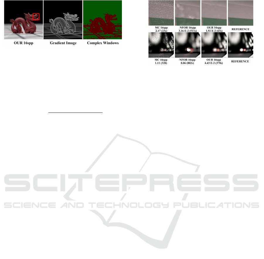
Figure 4: Window size selection. Our metric varies the win-
dow size based on area complexity.
pixel j computed from the model centered at pixel i.
To compute num, we follow the prior work (Liu
et al., 2017) of computing a Sobel gradient image in
the feature space, which showed that the Sobel op-
erator is sufficiently robust to recognize scene struc-
tures.:
gra
m
=
q
(G
x
∗
b
f
m
)
2
+ (G
y
∗
b
f
m
)
2
gra = max{gra
m
}
(14)
where gra is the gradient image computed as the max-
imum of gradient images gra
m
for each feature type.
G
x
and G
y
are the horizontal and vertical Sobel ker-
nels. num is computed as the number of pixels recog-
nized by gra in the same patch.
The result of our adaptive window selection is
shown in Fig.4. It is evident that the gradient image
extracted most fine details. In the third image of Fig.4,
we show the result by way of recognizing complex ar-
eas. The red pixels are recognized to be reconstructed
in a window of radius r
s
and the green pixels using
windows of larger radii. It is clear that our metric
varies the window size based on pixel complexity.
4 RESULTS AND DISCUSSION
We integrated our method as an extension with the
PBRT (Pharr and Humphreys, 2010) and employed
CUDA to accelerate our model. We used an Inter
CORE-i7 with 8 GB of RAM and a GeForce 650 M
GPU. Three state-of-the-art methods were used for
comparison: SBF (Li et al., 2012), WLR (Moon et al.,
2014), and NFOR (Bitterli et al., 2016). We used
rMSE (Rousselle et al., 2011) to measure numeri-
cal error (out − gt)
2
/(gt
2
+ ε), where out and gt are
the filtered value and the ground truth, respectively.
ε = 0.01 was used to prevent division by zero.
All images were rendered at a resolution of 800 ×
800 pixels. For our experiments, the patch size r
and threshold τ were set to 3 and 0.4, respectively.
The candidate window radii were set to {5,10,15}.
For our method, there are two parameters required to
be specified by users: sample number per pixel and
Figure 5: Comparisons between our algorithm and NFOR.
NFOR tended to blur fine details and failed to remove spike
noise.
the candidate bandwidth values (which were set to
k = {1.0,1.5,2.0,3.5,4.0} in our experiments).
4.1 Scenes
In Fig.5, we compare our method with NFOR. In
the second row of insets, it is clear that NFOR over
blurred image details while the results of our method
were closer to the reference image. Moreover, NFOR
could not remove spike noise (first row of insets) as
it dose not recognize outliers. Note that we intend
NFOR as a CPU-based method and, thus, it requires
a long time to complete reconstruction.
In Fig.6, the well-known ”SANMIGUEL” scene
containing complex geometries is compared in the
first two rows. SBF produced substantial noise at low
sampling rates, especially in background areas (the
first row of insets). It also failed to preserve fine detail
of the chair (second row of insets) because of inaccu-
rate SURE estimates. WLR outperformed SBF but
blurred details that did not have strong correlations
with the features. It did not weight the features appro-
priately either, leading to numerous splotches. Due to
the complementary strategy using the correlation be-
tween features and colors, our method performed bet-
ter. Our regression weights helped recognize details
that were not captured by the features and, thus, re-
turned clean details.
The last two rows of Fig.6 simulated two specific
rendering effects: depth of field and motion blur. It is
clear that both SBF and WLR failed to remove noise
in strongly defocused and motion-blurred areas. Our
method, however, provided robust input to fit data. As
a result, our method maintained the clarity of edges,
and was closer to the reference images.
4.2 Computational Overhead
To reduce cost, we wrote a GPU-based model for ac-
celeration. Moreover, The iterative number was set to
2 as it provided pleasing results in most cases. For
GRAPP 2018 - International Conference on Computer Graphics Theory and Applications
292

Figure 6: Comparisons of our method with prior methods.
our method, window size is varied at different pix-
els to further reduce cost. For example, only 34% of
the pixels were recognized to use small reconstruction
windows in the ”DRAGON” scene (Fig. 4). In this
case, each model of our method predicted 370 pixels
on average. Our method hence outperforms WLR at
the cost of a little more time.
4.3 Numerical Error Comparisons
To reduce the rMSEs, our method focuses on two
points. First, our prefiltering process removes feature
noise to produce a robust input for the model. Second,
we iteratively estimate and reduce the reconstruction
error at multiple pixels. In this case, as shown in Fig.5
and Fig.6, the lower numerical errors are produced. In
experiments, however, we also found that a relatively
large rMSE may be produced when our method failed
to recognize fine details from noise, especially for
scenes with complex geometries. We intent to solve
this problem by using novel features (e.g., visibility
and gradient) in our future work.
4.4 Limitations
A limitation of our method is that the correlation be-
tween features and colors may be not strong at low
sampling rates. Moreover, prefiltered features may be
overblurred and lead to blurred results. We believe
this problem can be solved by constructing a second
feature type (e.g., gradient) that is less influenced by
noise.
5 CONCLUSIONS AND FUTURE
WORK
To reduce the impact of noise, pixel colors are de-
noised using a GIF. In addition, we combine the joint-
NL-means filter with GIF to handle noisy features.
Our model uses an iterative process to estimate the
reconstruction error. Finally, the window size is se-
lected adaptively to reduce the computational over-
head. Experimental results demonstrate that the new
algorithm improves the image quality greatly and can
Denoising Monte Carlo Renderings based on a Robust High-order Function
293

handle a wide variety of rendering effects.
Overfitting to noise is a major challenge. Our
future work will extend the supervised learning ap-
proaches such as neural network. In addition, we in-
tend to compute the optimal bandwidth using a con-
sistent metric instead of selecting from a predefined
candidate set.
REFERENCES
Bako, S., Vogels, T., Mcwilliams, B., Meyer, M., Nov
´
aK,
J., Harvill, A., Sen, P., Derose, T., and Rousselle,
F. (2017). Kernel-predicting convolutional networks
for denoising monte carlo renderings. ACM Trans.
Graph., 36(4):97:1–97:14.
Belcour, L., Soler, C., Subr, K., Holzschuch, N., and
Durand, F. (2013). 5D covariance tracing for effi-
cient defocus and motion blur. ACM Trans. Graph.,
32(3):31:1–31:18.
Bitterli, B., Rousselle, F., Moon, B., Iglesias-Guitin,
J. A., Adler, D., Mitchell, K., Jarosz, W., and
Novk, J. (2016). Nonlinearly weighted first-order
regression for denoising Monte Carlo renderings.
Computer Graphics Forum (Proceedings of EGSR),
35(4):107117.
Chaitanya, C. R. A., Kaplanyan, A. S., and Schied, C.
(2017). Interactive reconstruction of monte carlo im-
age sequences using a recurrent denoising autoen-
coder. ACM Trans. Graph., 36(4):98:1–98:12.
Delbracio, M., Mus
´
e, P., Buades, A., Chauvier, J., Phelps,
N., and Morel, J.-M. (2014). Boosting Monte Carlo
rendering by ray histogram fusion. ACM Trans.
Graph., 33(1):8:1–8:15.
Durand, F., Holzschuch, N., Soler, C., Chan, E., and Sillion,
F. X. (2005). A frequency analysis of light transport.
ACM Trans. Graph., 24(3):1115–1126.
Egan, K., Hecht, F., Durand, F., and Ramamoorthi, R.
(2011). Frequency analysis and sheared filtering for
shadow light fields of complex occluders. ACM Trans.
Graph., 30(2):9:1–9:13.
Egan, K., Tseng, Y.-T., Holzschuch, N., Durand, F.,
and Ramamoorthi, R. (2009). Frequency analysis
and sheared reconstruction for rendering motion blur.
ACM Transactions on Graphics (SIGGRAPH 09),
28(3).
Hachisuka, T., Jarosz, W., Weistroffer, R. P., Dale, K.,
Humphreys, G., Zwicker, M., and Jensen, H. W.
(2008). Multidimensional adaptive sampling and re-
construction for ray tracing. ACM Trans. Graph.,
27(3):33:1–33:10.
He, K., Sun, J., and Tang, X. (2010). Guided image filter-
ing. In Proceedings of the 11th European Conference
on Computer Vision: Part I, ECCV’10, pages 1–14,
Berlin, Heidelberg. Springer-Verlag.
Kajiya, J. T. (1986). The rendering equation. In In: Pro-
ceedings of the 13th Annual Conference on Computer
Graphics and Interactive Techniques, SIGGRAPH
’86, pages 143–150, New York, NY, USA. ACM.
Kalantari, N. K., Bako, S., and Sen, P. (2015). A machine
learning approach for filtering monte carlo noise.
ACM Trans. Graph., 34(4):122:1–122:12.
Kalantari, N. K. and Sen, P. (2013). Removing the
noise in monte carlo rendering with general image
denoising algorithms. Computer Graphics Forum,
32(2pt1):93102.
Lehtinen, J., Aila, T., Chen, J., Laine, S., and Durand,
F. (2011). Temporal light field reconstruction for
rendering distribution effects. ACM Trans. Graph.,
30(4):55:1–55:12.
Li, T.-M., Wu, Y.-T., and Chuang, Y.-Y. (2012). Sure-
based optimization for adaptive sampling and recon-
struction. ACM Trans. Graph., 31(6):194:1–194:9.
Liu, Y., Zheng, C., Zheng, Q., and Yuan, H. (2017). Re-
moving monte carlo noise using a sobel operator and
a guided image filter. The Visual Computer.
Moon, B., Carr, N., and Yoon, S.-E. (2014). Adaptive
rendering based on weighted local regression. ACM
Trans. Graph., 33(5):170:1–170:14.
Moon, B., Iglesias-Guitian, J. A., Yoon, S.-E., and Mitchell,
K. (2015). Adaptive rendering with linear predictions.
ACM Trans. Graph., 34(4):121:1–121:11.
Moon, B., Jun, J. Y., Lee, J., Kim, K., Hachisuka, T., and
Yoon, S. (2013). Robust image denoising using a vir-
tual flash image for Monte Carlo ray tracing. Comput.
Graph. Forum, 32(1):139–151.
Moon, B., McDonagh, S., Mitchell, K., and Gross, M.
(2016). Adaptive polynomial rendering. ACM Trans.
Graph., 35(4):40:1–40:10.
Pharr, M. and Humphreys, G. (2010). Physically Based
Rendering: From Theory to Implementation. Morgan
Kaufmann Publishers Inc., San Francisco.
Rousselle, F., Knaus, C., and Zwicker, M. (2011). Adaptive
sampling and reconstruction using greedy error mini-
mization. ACM Trans. Graph., 30(6):159:1–159:12.
Rousselle, F., Manzi, M., and Zwicker, M. (2013). Robust
Denoising using Feature and Color Information. Com-
puter Graphics Forum.
Sen, P. and Darabi, S. (2012). On filtering the noise from
the random parameters in monte carlo rendering. ACM
Trans. Graph., 31(3):18:1–18:15.
Soler, C., Subr, K., Durand, F., Holzschuch, N., and Sillion,
F. (2009). Fourier depth of field. ACM Trans. Graph.,
28(2):18:1–18:12.
Zwicker, M., Jarosz, W., Lehtinen, J., Moon, B., Ra-
mamoorthi, R., Rousselle, F., Sen, P., Soler, C., and
Yoon, S.-E. (2015). Recent advances in adaptive sam-
pling and reconstruction for Monte Carlo rendering.
Comput. Graph. Forum, 34(2):667–681.
GRAPP 2018 - International Conference on Computer Graphics Theory and Applications
294