An Evolutionary Algorithm for an Optimization Model of Edge Bundling

Joelma Ferreira, Hugo Nascimento and Les Foulds

Institute of Informatics, Federal University of Goi

as, Alameda Palmeiras, Campus Samambaia, Goi

ania, Brazil

Keywords:

Edge Bundling, Optimization, Evolutionary, Approximate, Algorithm.

Abstract:

This paper presents two edge bundling optimization problems that address minimizing the total number of

bundles, in conjunction with other aspects, as the main goal. A novel evolutionary edge bundling algorithm for

these problems is described. The algorithm was successfully tested by solving two related problems applied

to real-world instances in reasonable computational time. The development and analysis of optimization

models have received little attention in the area of edge bundling. However, the reported experimental results

demonstrate the effectiveness and the applicability of the proposed evolutionary algorithm to help resolve edge

bundling problems formally deﬁned as optimization models.

1 INTRODUCTION

A graph is a mathematical structure for represent-

ing inherent relationships between objects. It is of-

ten drawn as a node-link diagram but, as the number

of elements increases, its ability to effectively display

information, without visual clutter, is a challenge.

Several existing graph drawing techniques attempt

to reduce visual clutter. An example is edge bundling,

which has gained attention as a way to improve the

readability of a graph drawing by merging geometri-

cally close edges into bundles along a shared path.

Traditional edge bundling approaches are

not problem-speciﬁc methods but instead, are

application-oriented. They are not dedicated to solve

a mathematically-formulated problem, i.e., they do

not follow a systematic and theory-guided process

to propose and solve edge bundling optimization

problems by deﬁning decision variables and a given

objective function to be optimized.

The consequence is that those approaches do not

address the issue of identifying the “best” set of bun-

dles based on a group of criteria that are mathemati-

cally deﬁned in the form of an objective function.

Conversely, in a previous paper (Ferreira et al.,

2017), edge bundling was formally deﬁned and in-

vestigated as an optimization problem for the ﬁrst

time. Speciﬁcally, it was formulated as a constrained

combinatorial optimization problem in which the to-

tal number of bundles is to be minimized and only

edges with a common node

can be bundled together.

Edges with a common node are termed “adjacent” and

The problem of bundling only adjacent edges appears

to provide a better sense of proximity between edges

and nodes and has been shown to be NP-hard. A

more advanced problem was also deﬁned by impos-

ing a maximum angle (α) constraint between any pair

of adjacent edges to be bundled. Therefore, the prob-

lem became minimizing the number of edge bundles

while respecting the α-angle constraint. It is termed

the Angle-Based Edge Bundling Problem (ABEB).

Ferreira et al. (2017) highlights how complex and rel-

evant edge bundling optimization is.

In the present paper, we continue the investigation

into the formal modeling of edge bundling and pro-

pose a third problem. The new problem is denoted

as the Compatibility-Based Edge Bundling Problem

(CBEB) and it involves minimizing the total number

of bundles while maximizing a multi-objective func-

tion that incorporates well-known edge compatibil-

ity measures. We also propose an approximate evo-

lutionary algorithm, called here Evolutionary Edge

Bundling (EEB), for ABEB and CBEB. As far as we

know, EEB is the ﬁrst heuristic method ever proposed

for these problems

Experiments with the evolutionary algorithm

show that it produces close-to-optimal solutions for

some of the nontrivial ABEB instances tested. The

results reinforce the importance of optimization ap-

proaches for edge bundling, not only as a way of vi-

sualizing a graph with less visual clutter, but also as a

those without are termed “nonadjacent’.

Ferreira et al. (2017) presented only an integer linear

formulation for the ABEB, not a solution method.

132

Ferreira, J., Nascimento, H. and Foulds, L.

An Evolutionary Algorithm for an Optimization Model of Edge Bundling.

DOI: 10.5220/0006626901320143

In Proceedings of the 13th International Joint Conference on Computer Vision, Imaging and Computer Graphics Theory and Applications (VISIGRAPP 2018) - Volume 3: IVAPP, pages

132-143

ISBN: 978-989-758-289-9

way of systematically studying and comparing prob-

lem deﬁnitions, methods and solutions in this ﬁeld.

From now on, we consider only undirected graphs.

The remainder of the paper is organized as fol-

lows. Section 2 brieﬂy surveys relevant work on var-

ious aspects of edge bundling. Section 3 presents a

deﬁnition of edge bundling as a combinatorial op-

timization problem, as proposed in (Ferreira et al.,

2017). Some compatibility and aesthetic criteria used

as constraints and as part of the objective function of

our problems are then discussed in Section 4. Sec-

tion 5 provides the formal deﬁnitions of ABEB and

CBEB. Section 6 introduces the evolutionary edge

bundling algorithm aimed at solving these two prob-

lems and Section 7 describes the experimental results.

Section 8 discusses a method (EEB) for rendering the

edge bundling solutions as a ﬁnal step of the edge

bundling process. A comparison of EEB with pre-

vious edge bundling techniques is discussed in Sec-

tion 9. Finally, in Section 10, we draw some conclu-

sions and discuss ideas for future research.

2 RELATED WORK

The scientiﬁc literature on edge bundling is exten-

sive and reports many edge bundling techniques. For

instance, the approach developed by Holten (2006),

called hierarchical edge bundling, uses hierarchy tree

branches for edge routing; in (Cui et al., 2008), a

method called geometric edge bundling forms bun-

dles by routing edges along a mesh generated by

a triangulation algorithm; the force-directed edge

bundling technique (Holten and van Wijk, 2009; Se-

lassie et al., 2011) splits the edges into segments that

attract each other as a basis for bundling edges; the

skeleton-based edge bundling method (Ersoy et al.,

2011) generates a skeleton from the medial axes of

groups of similar edges, and then attracts edges to

this skeleton; and the kernel density estimation edge

bundling method (Hurter et al., 2012) computes a den-

sity map and moves the edges in the gradient direction

of where the bundles will be formed.

Those and many other edge bundling techniques

attempt to aggregate edges with similar properties

into bundles, addressing mainly the question of spec-

ifying how these edges should be routed along the

same path. The techniques produce solutions in

which the coarse structure of the graph is revealed

but fail to show connection patterns at the node level.

Peng et al. (2012) afﬁrm that sometimes, it is more

important to show the connection trends of a node

rather than the overall network structure. For ex-

ample, in graph drawings representing a route net-

work, the actual relationships between interconnected

components are usually more relevant than the coarse

structure of the graph. This happens because many

traditional edge bundling methods generate bundles

that have common interior segments and multiple

source and destination nodes, i.e., they “knot” the

edges in the middle of the bundle.

Consequently, Peng et al. (2012) proposed an al-

gorithm called node-based edge bundling that bun-

dles and “knots” edges nearer to the common node

of adjacent edges. Nocaj and Brandes (2013) reﬁned

the technique of (Peng et al., 2012) and proposed a

method called stub bundling that joins only edges that

share the same endpoint with the aim of visualizing

unambiguous graphs and retrieving the exact source

and target of each edge. Their method uses the angle

between consecutive edges as the criterion for choos-

ing which edges to be joined together.

Even though the methods of Peng et al. and No-

caj and Brandes efﬁciently produce bundles with only

adjacent edges, neither of them has the aim of explic-

itly minimizing the number of bundles. In order to

achieve this goal, the formulation of an optimization

problem is required, deﬁning decision variables, con-

straints and objectives. In order to address the afore-

mentioned need, the present paper investigates the

problem of ﬁnding the “best” conﬁguration of bun-

dles (involving only adjacent edges) that maximizes a

given objective function.

3 EDGE BUNDLING AS AN

OPTIMIZATION PROBLEM

There is a present lack of fundamental and theoretical

principles that can be used to objectively measure the

effectiveness of bundling techniques. Despite some

attempts to formalize the presentation of certain edge

bundling methods, bundling itself, as a technique, as

yet lacks an underlying formalism that can unify pre-

vious methods. Most existing edge bundling deﬁni-

tions are vague, each related to slightly different char-

acteristics of the problem. Moreover, edge bundling

is related to both joining edges and determining the

paths of the edges.

Recently, McKnight (2015) and Lhuillier et al.

(2017) have discussed those complementary aspects

when presenting more complex mathematical formu-

lations of edge bundling. McKnight deﬁnes a bun-

dle as a set of two or more “edge segments”, and

edge bundling as the decision of how to segment the

edges. Lhuillier et al. (2017) deﬁne a bundle as a set

of paths that share similarities and edge bundling as

the method that creates bundles and trails.

An Evolutionary Algorithm for an Optimization Model of Edge Bundling

133

McKnight (2015) afﬁrms that many existing edge

bundling approaches do not generate bundles directly.

In fact, for most edge bundling algorithms, the out-

put is just a graph drawing and the search for a good

layout is a heuristic based on an informal or implicit

deﬁnition of the desirable optimization goals.

Consequently, we take a different direction by for-

mally deﬁning edge bundling as an optimization prob-

lem. We also aim at a solution that has a bundle con-

ﬁguration as an output. For the structure of the solu-

tion, we follow the deﬁnition given by McKnight that

focus on computing bundles directly, but we consider

a bundle as a set of edges (not a set of edge segments

as McKnight does).

Thus, in (Ferreira et al., 2017), edge bundling was

formulated as an optimization problem that attempts

to ﬁnd the “best” set of bundles in terms of some given

parameters, goals and constraints. A general edge

bundling optimization problem, that can be used as

a framework for describing more speciﬁc problems,

was deﬁned as follows:

Deﬁnition 1. Let G = (V,E) be a graph and D a given

unbundled node-link drawing of G in the plane. Con-

sider S = (E

,...,E

) a partition of E (not nec-

essarily disjoint), n ∈ N

. Further, let R be a func-

tion that takes G, D and S, and renders a bundled

graph drawing version of D called D

, given some

extra necessary information, such as rules for rout-

ing the edges. The general edge bundling problem is

hence to determine the partition S (here called bun-

dles), with E = ∪

i=1

, so that, a set F of objective

functions, representing aesthetic edge bundling mea-

surements of D

, are optimized (minimized or max-

imized), and a set P of constraints (deﬁning mainly

which edges can be bundled together) are satisﬁed.

Note that Deﬁnition 1 enables the inclusion of the

routing problem

as a question to be addressed by

the optimization problem. This can be done in two

ways: (1) by solving the routing as a second-level

problem totally inside the rendering function R; or (2)

by extending the formal deﬁnition in order to have

extra variables that determine the routing and that are

used in R. In both cases, functions that evaluate the

quality of the resultant edge-bundling drawings, pro-

duced by R, can be included in the set F, making the

edge-routing problem more intrinsic to the optimiza-

tion process. Some quality aspects that may inﬂuence

the routing, such as minimizing the amount of ink

for drawing the bundles, or minimizing the amount

of edge crossings, can be pursued using these ap-

proaches. However, in the present paper, the routing

Deﬁning the precise paths on which the bundled and

possibly the unbundled edges travel through.

problem is not considered critical for the optimization

process. Therefore, it was treated as a fully indepen-

dent problem (see (1) above) and was considered an

external, post-processing stage (see Section 8).

4 COMPATIBILITY AND

AESTHETICS

The terms “compatibility” and “aesthetics” suggest

preferable features that a layout should possess, in or-

der to help to reduce visual clutter. These features are

important aspects of the EEB framework, since they

determine the constraints and objectives of the prob-

lems being investigated. In the next two subsections,

some measures used in the evolutionary algorithm for

obtaining such features are detailed, and some aes-

thetics for edge bundling are discussed.

4.1 Compatibility Measures

Generally, edge bundling techniques decide which

edges will be bundled together (Holten and van Wijk,

2009; Nguyen et al., 2011). The proposed evolution-

ary formulation focuses on two measures introduced

by Holten and van Wijk (2009)

: Angle compati-

bility, C

∈ [0, 1], that avoids joining perpendicular

edges; and Scale compatibility, C

∈ [0,1], which

prevents joining edges that differ in length. The to-

tal compatibility, C ∈ [0, 1], between two edges is

C = C

×C

4.2 Aesthetics for Edge Bundling

A graph drawing method usually tries to produce

drawings that are considered visually pleasing, ac-

cording to speciﬁc aesthetic criteria, for example,

minimizing the number of edge crossings or maxi-

mizing the number of symmetries, etc (Battista et al.,

1998). However, most of the known heuristics for

edge bundling are not necessarily involved with the

exploration and evaluation of the quality of a drawing

with respect to such aesthetics.

There are few reported attempts to incorporate

and optimize aesthetic criteria in edge bundling lay-

outs. Recently, Angelini et al. (2016) restricted edge

bundling to the end segments of edges and allowed at

most one crossing per bundle. Alam et al. (2016) pro-

posed a formulation focused on minimizing the num-

ber of bundled crossings for circular graphs but no

Holten and van Wijk (2009) proposed two other mea-

sures, position and visibility, but they were not explicitly

employed in our approach because they are covered by the

adjacency constraint.

IVAPP 2018 - International Conference on Information Visualization Theory and Applications

134

proof of its NP-completeness, nor an approximation

algorithm were presented. Saga (2016) proposed two

measures to quantitatively evaluate edge bundling:

edge lengths and area occupation. The effectiveness

of those measurements was not discussed.

We believe that, besides reducing the clutter,an

edge bundling technique could potentially improve

the readability of a graph drawing if it was con-

structed to optimize one or more aesthetic criteria

related to the bundling structure. As a result, edge

bundling could possibly be formalized as a multi-

objective optimization problem, where the layout is

generated according to a given set of aesthetics. We

propose and attempt to implement strategies for some

of the following edge bundling aesthetic criteria:

(i) minimizing the total number of bundles;

(ii) maximizing the compatibility of bundled edges;

(iii) maximizing the number of edges per bundle;

(iv) minimizing the ambiguity of the edges;

(v) maximizing the axial symmetry of the bundles;

(vi) minimizing the total number of crossings between

edges and/or bundles.

5 EDGE BUNDLING PROBLEMS

In this paper, two edge bundling problems are inves-

tigated that tightly combine Deﬁnition 1 with some

aesthetics and compatibility measures.

Problem 1 (Angle-Based Edge Bundling Problem

(ABEB)). Given a drawing D of a graph G = (V,E),

a function γ

that returns the smaller angle

be-

tween any pair of adjacent edges e

and e

from E in

the drawing, and an angle α, 0 ≤ α ≤ 180

◦

, the ABEB

problem

is to determine a partition of E into disjoint

subsets E

,. .. ,E

, E = ∪

i=1

, that minimizes n,

subject to each E

inducing a star subgraph G

(i.e,

all edges in E

share a same node), and γ

i j

≤ α for

every two edges e

i j

, e

∈ E

ABEB is the original problem proposed in (Fer-

reira et al., 2017). Note that a set E

represents a bun-

dle containing only adjacent edges, and that each edge

of the graph appears in exactly one bundle.

For a given input graph drawing, there may be

many solutions with the same number of bundles and

We deﬁne the smaller angle as the lesser angle be-

tween two adjacent edges with regard to the clockwise and

counter-clockwise orientations between the edges.

The original name of this problem is EB−star

but, for

the sake of clarity, it will be called ABEB here.

satisfying the angle constraints, but with a different

composition of the sets E

,. .. ,E

. In order to

distinguish between these solutions, the additional

objective of maximizing the compatibility value be-

tween edges is added to the original ABEB. The aim

is to produce solutions in which the edges in E

are as

compatible as possible. The precise deﬁnition of this

new problem is given below.

Problem 2 (Compatibility-Based Edge Bundling

Problem (CBEB)). Let D be a drawing of a graph

G = (V, E). For D, let C(a,b) be the compatibil-

ity measure between each pair of edges a,b ∈ E

(as previously deﬁned in Section 4.1), and C

∑

p,q∈E

C(p,q) the total compatibility of a bundle E

deﬁned as the sum of C for all pairs of edges in the

bundle. The CBEB problem is to determine a partition

of E into disjoint subsets E

,. .. ,E

, E = ∪

i=1

that maximizes C

∑

i=1

and minimizes n, sub-

ject to each E

inducing a star subgraph G

Thus, CBEB has two objectives: to maximize the

sum of the compatibilities of the edge bundles and

to minimize the number of edge bundles. These ob-

jectives may balance each other out when ﬁnding a

minimal set of bundles. For the purpose of simpli-

ﬁcation, CBEB was converted into a single-objective

problem aimed at maximizing the following weighted

sum function:

f = w

×C

+ w

(1)

where 0 ≤ w

≤ 1, i = 1,2.

Note that the angle limit α is not a constraint of

the problem any more, but angle compatibility is part

of the objective function, embedded in C

6 EVOLUTIONARY EDGE

BUNDLING (EEB)

One of the challenges of dealing with difﬁcult com-

binatorial optimization problems is to develop algo-

rithms that guarantee to ﬁnd a reasonably good solu-

tion in an acceptable computational time. A technique

that has frequently been able to address this challenge

successfully in many situations is so-called evolution-

ary computation, a generic population-based approx-

imate metaheuristic optimization algorithm from arti-

ﬁcial intelligence. An evolutionary algorithm (B

ack,

1996) (EA) is a subset of evolutionary computation,

An EA uses mechanisms inspired by biological evolu-

tion, such as reproduction, mutation, recombination,

and selection.

An Evolutionary Algorithm for an Optimization Model of Edge Bundling

135

Following that line, we present a novel EA for the

edge bundling problems ABEB and CBEB. The algo-

rithm adopts the standard evolutionary cycle involv-

ing population initialization, evaluation, selection, re-

combination and mutation steps. The next subsec-

tions describe the solution representation and details

of the steps of the algorithm.

6.1 Representation Scheme

Given a graph G = (V,E), the representation of an

edge bundling solution (also called here an individ-

ual of a population) for ABEB (or CBEB) is simply

I = (E

, E

, ..., E

), that is, the sets of bundles of

edges E

⊂ E (1 ≤ i ≤ n), 1 ≤ |E

| ≤ |E|. The cardi-

nality of individuals is variable, but cannot exceed a

given maximum cardinality, n ≤ |E|. Constraint sat-

isfaction is an integral part of the concept of a genetic

operator. Therefore, we assume that the sets E

are

disjoint and that E = ∪

i=1

as speciﬁed by ABEB

(CBEB). Figure 1 illustrates the representation of a

simple bundled graph with four bundles E

and

. The bundle E

, for example, is composed of the

edges 1, 2 and 3. The routing of the edges and other

visual aspects of the bundling are not included in our

current solution representation. These elements are

treated automatically by a rendering function at the

last stage of the edge bundling process.

1, 2, 3 4, 5 6, 7, 8 9, 10

E1 E2 E3

Bundled Gr aph

Repr esentati on

Figure 1: Individual representation scheme.

6.2 Fitness Function

The quality of each individual is evaluated according

to a ﬁtness function. This function is simply a max-

imization version of the objective function required

to be optimized in either ABEB or CBEB (see Sec-

tion 5). For the CBEB case, an adaptation was done

via the f function, in order to further penalize solu-

tions with bundles having very low compatibility val-

ues. For this, the thresholds T

and T

were deﬁned,

representing lowest acceptable values for C

and C

respectively. Then, for the pair of edges p, q ∈ E

that

induces the smallest compatibility C(p, q) among all

other pairs in E

, if C

(p,q) < T

or C

(p,q) < T

then

is set to -1.

6.3 Initialization

In order to explore the search space at points that

are distributed as evenly as possible, two methods

for generating the initial population were devised.

The ﬁrst method is a heuristic method based on solu-

tions for the minimum vertex cover problem (Skiena,

1990), while the second algorithm selects the initial

population randomly using pseudo-random numbers.

Each method generates half of the initial population.

In the ﬁrst strategy, a minimal vertex cover set A

of V is generated by a heuristic process. Then, each

node v ∈ A is considered as the center of an induced

star subgraph in G. Finally, edge bundling sets are

created, each one taking edges from a randomly cho-

sen star subgraph. The edges that comprise a bun-

dle are also chosen at random, but only compatible

edges, (relative to a given threshold) can be joined

together. For the ABEB and CBEB problems, the

threshold represents the maximum value of the de-

sired constraints (maximum angle and/or minimum

compatibility measures). This approach was found to

be effective, usually generating individuals near the

optimal solution (related to the number of bundles) for

populations of large size. However, preliminary ex-

periments also showed that a population created using

only this method can lead to premature convergence.

In order to address the problem of premature con-

vergence, the other strategy initializes the second half

of the population randomly. It creates individuals by

randomly choosing adjacent edges to create bundles,

while still ensuring feasibility and threshold satisfac-

tion. As a consequence, this method can produce un-

interesting individuals but it facilitates an increase in

population diversity.

After an individual is generated, both strategies

enable bundles to be shufﬂed in their positions. This

improves the efﬁciency of the crossover operator, cre-

ating more interesting random individuals and also

preventing premature convergence.

If any individual is found duplicated, a removal

function is used to replace or discard it. We use the

approach of Saroj (2012) in which any duplicated in-

dividual is replaced probabilistically with a mutated

version of the best individual presented in the popula-

tion. After applying a test, if the individual is still du-

plicated, then it is discarded. A checksum (based on

the number of bundles, on the edges present in each

bundle, and on the ﬁtness) is used to quickly check

the solution. The checksum is invariant with regard to

the position of the bundles in the representation.

IVAPP 2018 - International Conference on Information Visualization Theory and Applications

136

6.4 Selection

The strategy used for randomly selecting individu-

als for recombination is tournament selection with re-

placement. In addition, after recombining two indi-

viduals and mutating their two offspring, the steady

state is applied, where the offspring produced com-

pete for survival against the members of the current

population. This is done by inserting the newborn

offspring in the current population and removing the

worst two individuals. After repeating this process

t times, where t is the number of individuals in the

population, the best individual of the last generation

is propagated to the new one, if it has a higher ﬁtness.

If this happens, the best individual randomly replaces

a solution in the resultant population.

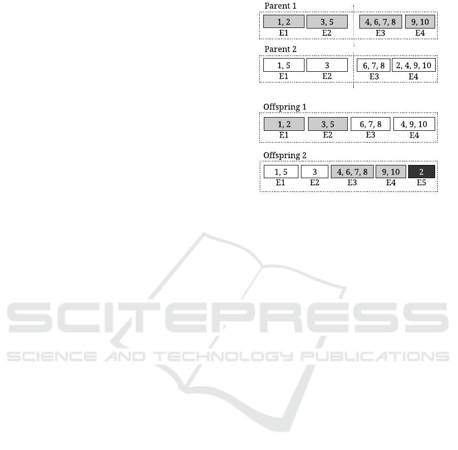
6.5 Crossover Operator

The one-point and two-point classic methods are ap-

plied (they are chosen randomly each time) to pro-

duce the recombination of the parental sets of bun-

dles. This is accomplished by swapping the list of

bundles of two parents in order to create a new ran-

dom set I, representing two new individuals. First,

the crossover points are selected. In the one-point

crossover, the selected point is at the middle part of

the smallest parent (the smallest n value divided by

two). The right-hand side of the parents are then

swapped (see Figure 2). In the two-point crossover,

the points are also deﬁned by the size of the smallest

individual, dividing it in three equall-sized parts. The

middle parts are then swapped.

During the crossover process, infeasible offspring

(that violate the disjoint-set constraint or do not cover

all edges) may be produced and need to be repaired.

Thus, the latest occurrence of duplicated edges are re-

moved and missing edges are inserted in new solitary

bundles in the ﬁnal solution representation. This is il-

lustrated in Figure 2, where edge 2 was removed from

bundle E

in Offspring-1, and the same edge was in-

serted in a new bundle in Offspring-2.

6.6 Mutation Operators

The mutation operators speciﬁed for EEB are:

• Join mutation randomly selects two solitary bun-

dles and merges them if their edges are adjacent.

• Merge mutation is similar to Join mutation. The

difference is that it works with bundles of any size

and only the ﬁrst bundle is chosen at random. The

other merged bundle is the ﬁrst compatible one

found by a sequential search in the representation

of the individual.

1, 2

3, 5

6, 7, 8 4, 9, 10

Offspr ing 1

1, 5 3 4, 6, 7, 8 9, 10

E2 E3 E5

Offspr ing 2

1, 2

3, 5 4, 6, 7, 8 9, 10

E1 E2

1, 5 3

6, 7, 8

2, 4, 9, 10

E1 E2

Par ent 2

Par ent 1

Figure 2: A example of one point crossover operation.

• Split mutation replaces a randomly chosen bun-

dle by dividing it into two subbundles.

• Move mutation randomly selects a bundle and

moves one of its edges to another the ﬁrst com-

patible bundle found.

• Remove mutation randomly removes an edge

from a bundle of size greater than one and creates

a new solitary bundle with that edge.

The mutation operation to be used is chosen at

random each time. There is also a constant proba-

bility of applying it.

7 EXPERIMENTAL RESULTS

Experiments for testing our approach EEB were con-

ducted with one synthetic graph and eight real-world

graphs. The graphs are: Synthetic (G1 – 20 nodes,

28 edges) (Ferreira et al., 2017), ZacharyClub (G2 –

34 nodes, 78 edges) (Zachary, 1977), PlanarGD2015

(G3 – 66 nodes, 101 edges) (ISGCI, 2015), Dolphin

(G4 – 62 nodes, 160 edges) (Girvan and Newman,

2002), a connected version of MovieLens (G5 – 160

nodes, 161 edges) (MovieLens, 2017), LesMiserables

(G6 – 77 nodes, 254 edges) (Knuth, 1993), Book-

sUSPolitics (G7 – 105 nodes, 401 edges) (Newman,

2006), Flare Software Class (G8 – 220 nodes, 709

edges) (Holten, 2006) and the USAirline (G9 – 235

nodes, 1297 edges) from an unknown source.

We executed two sets of experiments, one for each

of the ABEB and CBEB problems discussed in Sec-

tion 5. The initial layout of the graphs with ﬁxed

nodes was predeﬁned in an input ﬁle. The exper-

iments consisted of running the evolutionary algo-

An Evolutionary Algorithm for an Optimization Model of Edge Bundling

137

Table 1: Results for the ABEB problem, averaged over 100 independent runs, u = 150, p

= 0.98 and p

= 0.4.

Graph Edges α(

◦

) Bundles of Avg. Avg. Std. dev. Std. error Avg.

best solution bundles ﬁtness ﬁtness ﬁtness time (s)

G1 28

30 17 (100) 17.00 0.0588 0.00000 0.000000 2

45 16 (100) 16.00 0.0625 0.00000 0.000000 1

70 13 (89) 13.11 0.0763 0.00173 0.000173 1

G2 78

30 45 (1) 49.74 0.0201 0.00073 0.000073 6

45 37 (3) 39.75 0.0252 0.00081 0.000081 6

70 31 (6) 33.30 0.0301 0.00101 0.000101 5

G3 101

30 75 (4) 76.84 0.0130 0.00015 0.000015 9

45 69 (1) 73.01 0.0137 0.00023 0.000023 9

70 60 (4) 62.63 0.0160 0.00028 0.000028 9

G4 160

30 107 (4) 111.08 0.0090 0.00019 0.000019 20

45 92 (6) 96.57 0.0104 0.00026 0.000026 19

70 75 (2) 79.48 0.0126 0.00032 0.000032 18

G5 161

30 65 (2) 69.28 0.0144 0.00028 0.000028 11

45 51 (1) 54.17 0.0185 0.00050 0.000050 11

70 37 (1) 40.84 0.0245 0.00085 0.000085 10

G6 254

30 121 (4) 128.23 0.0078 0.00022 0.000022 156

45 99 (1) 107.13 0.0093 0.00032 0.000032 40

70 82 (4) 88.01 0.0114 0.00039 0.000039 29

G7 401

30 238 (1) 251.82 0.0040 0.00009 0.000009 101

45 207 (1) 217.45 0.0046 0.00010 0.000010 88

70 169 (2) 178.71 0.0056 0.00014 0.000014 66

G8 709

30 339 (1) 354.39 0.0028 0.00006 0.000006 198

45 280 (3) 293.35 0.0034 0.00008 0.000008 167

70 235 (2) 247.62 0.0040 0.00009 0.000009 167

G9 1297

30 338 (1) 355.85 0.0028 0.00008 0.000008 524

45 281 (1) 295.32 0.0034 0.00009 0.000009 451

70 221 (1) 236.72 0.0040 0.00012 0.000012 420

rithm for 100 independent trials for each graph and

angle parameter. For the ABEB, the angle parame-

ter was progressively ﬁxed as α = 30

◦

,45

◦

,70

◦

. For

the CBEB, the angle parameters were considered, but

they were employed for calculating T

thresholds us-

ing the formula T

= 1 −α/180. Furthermore, for the

CBEB, the weights of the components of the objec-

tive function were chosen empirically as w

= 0.2 and

= 0.8 (see Section 5). Other parameters deﬁned

for both sets of experiments were: the population size

(u = 150), the crossover rate (p

= 0.98), and the mu-

tation rate (p

= 0.4). The evolutionary cycle was

repeated until there was no further improvement in

the population for 500 consecutive iterations or the

maximum number of generations (set at 16,500) was

achieved. All tests were executed on a MacBook Pro

with an Intel Core i7 processor of 2.9 GHz and 8GB

of 1600MHz-DDR3 RAM.

7.1 Results for the ABEB Problem

The ﬁrst experiment aimed to produce solutions with

the minimum number of bundles, and all edge angles

in a bundle never higher than a given α. Table 1 sum-

marizes the results for the various graphs. The ﬁrst

three columns consist of general information. The

fourth column shows the number of bundles of the

best solution in 100 trials. The amount of trials in

which a solution with that quality appeared is pre-

sented in parenthesis. The ﬁfth and the sixth columns

present the average values of the number of bundles

of the best solutions, and the average of their ﬁtness,

respectively, over the 100 trials. The seventh and the

eight columns are the standard deviation and the stan-

dard error of the ﬁtness values. The last column shows

the average of the total runtime.

Analyzing the table, one can see that the average

of the number of bundles in the best solutions was

nearby the best one found over the independent trials.

In addition, the standard deviations were low, indicat-

ing that a majority of the generated solutions are po-

sitioned close to the mean ﬁtness. Figure 3 illustrates

the best solutions obtained for the graph G5 with an-

gle constraints α = 30

◦

and α = 70

◦

. A comparison

between Figures 3(a) and (b) shows the effect on the

bundling as the α angle increases, joining more edges.

This is very noticeable for the edges connected to the

highlighted nodes (drawn as circles in light yellow).

In general, when solving the ABEB, the EEB

method produced good results in terms of the number

IVAPP 2018 - International Conference on Information Visualization Theory and Applications

138

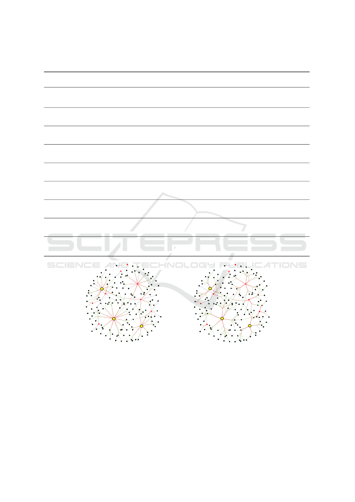
Table 2: Results for the CBEB problem, averaged over 100 independent runs, u = 150, p

= 0.98, p

= 0.4, w

= 0.2,

= 0.8 and T

= 0.890.

Graph Edges α(

◦

) Bundles of Avg. compa- Avg. Avg. Std. dev. Std. error Avg.

best solution tibility bundles ﬁtness ﬁtness ﬁtness time (s)

G1 28

30 20 (3) 9.48 20.01 1.9354 0.02551 0.002551 2

45 16 (2) 13.27 18.17 2.6990 0.29839 0.029839 2

70 16 (2) 20.22 16.82 4.0925 0.24830 0.024830 2

G2 78

30 56 (2) 22.69 58.49 4.5518 0.24592 0.024592 11

45 48 (1) 35.87 50.72 7.1901 0.49003 0.049003 13

70 36 (1) 69.97 39.10 14.0145 0.86055 0.086055 15

G3 101

30 81 (1) 23.23 83.86 4.6546 0.33595 0.033595 12

45 76 (1) 34.94 81.10 6.9985 0.80816 0.080816 13

70 65 (1) 84.31 69.05 16.8739 0.61844 0.061844 18

G4 160

30 129 (1) 29.49 132.78 5.9044 0.40687 0.040687 31

45 112 (1) 50.48 119.24 10.1020 0.66873 0.066873 39

70 89 (1) 108.68 94.89 21.7440 1.45149 0.145149 47

G5 161

30 76 (1) 136.71 83.90 27.305 2.18483 0.218483 33

45 60 (1) 218.55 69.79 43.7209 4.24025 0.424025 36

70 50 (1) 387.42 52.88 77.5001 5.80255 0.580255 35

G6 254

30 174 (1) 121.04 180.17 24.2121 2.08592 0.208592 103

45 137 (1) 206.14 147.32 41.2327 3.00882 0.300882 111

70 97 (1) 426.76 101.97 85.3606 4.74743 0.474743 101

G7 401

30 305 (1) 170.56 312.62 34.1143 1.68656 0.168656 300

45 260 (1) 266.62 270.62 53.3276 2.48894 0.248894 315

70 209 (1) 501.12 213.89 100.2274 4.68943 0.468943 363

G8 709

30 452 (1) 410.16 464.50 82.0344 4.58910 0.458910 684

45 379 (1) 663.31 395.09 132.6634 4.62701 0.462701 834

70 312 (1) 1108.79 318.49 221.7608 9.51946 0.951946 828

G9** 1297

30 530 (1) 2159.99 535.93 431.9990 14.91452 3.986073 18551

45 428 (1) 3249.19 437.40 649.8400 22.67482 5.854614 11110

70 318 (1) 5774.74 327.73 1154.9496 57.56356 14.862847 6859

(a)

(b)

Figure 3: MovieLens (G5) for ABEB with different angle constraints, (a) α = 30

◦

and (b) α = 70

◦

of bundles and the α angle constraint. On the other

hand, some bundles may have edges that differ signif-

icantly in length. Therefore, as expected, the ABEB

usually produces bundles with low scale compatibil-

ity between the edges.

7.2 Results for the CBEB Problem

The second experiment was conducted in order to im-

prove the results by introducing the compatibility cri-

teria (CBEB). Table 2 summarizes the experimental

results for this problem. It follows the same struc-

ture as Table 1 and includes one column representing

the average compatibility measure of the best solu-

tions in 100 trials. The stochastic nature of the al-

An Evolutionary Algorithm for an Optimization Model of Edge Bundling

139

(a)

(b)

Figure 4: LesMiserables (G6) with α = 70

◦

, (a) ABEB solution with 82 bundles and (b) CBEB solution with 97 bundles.

gorithm associated with the size of the search space

produced solutions signiﬁcantly different from each

other in terms of ﬁtness. However, the standard error

reﬂects a low sampling ﬂuctuation. Note that similar

results did not occur for the USAirline (G9) graph,

ﬁrst because the experiment was repeated only for 15

independent trials for this graph and also because the

number of edges signiﬁcantly increased the size of the

search space. These results highlight how the number

of edges can dramatically increase the set of candidate

solutions for the CBEB problem.

Figure 4(b) shows the best solution produced by

EEB for the LesMiserables (G6) graph for the CBEB.

Note that, although the number of bundles has in-

creased, the solution for CBEB has bundles having

more similar edges than the solution produced for

ABEB (Figure 4(a)). The ﬁgures show that some

bundles present in the ABEB solution split and some

other were created in the CBEB solution.

Another additional feature of the CBEB is that, as

a multi-objective problem, the solution with the low-

est number of bundles is not always produced. This is

because the ﬁnal solution depends on the weights in

the objective function and on the compatibility values

of the current results.

7.3 Comparison of EEB and an Exact

Approach for ABEB Problem

We now establish a qualitative point of view of the

complexity of the edge bundling problems discussed

in this paper and attempt to show that the EEB al-

gorithm is a promising approach. To do this, we

present (in terms of number of bundles and runtime

execution) the best solution over 100 independent ex-

ecutions obtained by EEB for the graphs Synthetic

and PlanarGD2015 for the ABEB problem. We then

compare numerical results with those generated by an

exact method based on an integer programming (IP)

model for the ABEB problem, published in (Ferreira

et al., 2017). The exact method is implemented using

Table 3: Comparison of number of bundles generated by

EEB with an exact method (IP) for ABEB problem.

Graph Edges α(

◦

) EEB IP Time Time

EEB (s) IP (s)

G1 28

30 17 17 2 0.16

45 16 16 1 0.16

70 13 13 1 0.35

90 11 11 1 0.39

110 10 10 1 0.14

G3 101

30 75 74 9 125.65

45 69 69 9 656.14

70 60 58 9 1210.29

90 53 50 9 1275.27

110 48 - 9 -

the Gurobi solver (Optimization, 2017) and a more

powerful computer (a DELL M630 server with 128

GB of RAM and 2 processors with 10 cores each –

40 visible cores of 3-3.6Ghz). The EEB method ran

on the simpler computer previously described. More

alpha angles were used this time. The results are

reported in Table 3. The fourth and ﬁfth columns

present the number of bundles of the best solutions

by EEB and the exact IP method, respectively. A line

with a dash means that no solution was produced by

the IP method even after several hours of runtime.

The values in table show that the IP method was

effective in generating the optimal solutions only

for small numerical instances and took an inordinate

amount of time to solve some of the larger instances.

For the graph G3 with 101 edges the IP method failed

with a maximum angle of 110

◦

, implying that the ex-

act method is not practical for medium-sized ABEB

and CBEB problems as it requires excessive compu-

tation time.

Conversely, the EEB approach was usually suc-

cessful in ﬁnding close-to-optimal solutions. In addi-

tion, the execution time of EEB is signiﬁcantly lower

than that of the IP method for the larger graphs, even

when using a less powerful computer.

IVAPP 2018 - International Conference on Information Visualization Theory and Applications

140

8 VISUALIZATION

Most existing edge bundling methods draw edges in-

dividually and route them closely. In contrast, the

EEB approach only outputs sets of edges representing

bundles. Those groups of edges form star subgraphs.

After the evolutionary algorithm has terminated, the

subgraphs of the best-found solution can then be sub-

mitted to a rendering module for producing an edge

bundling drawing.

In order to allow an adequate visual interpretation

of the EEB results, mainly the comprehension of the

relation patterns between the nodes, two visualiza-

tions are proposed in the present work. The ﬁrst one

shows bundled edges as a colored cubic B

ezier curve,

going from red to green by default. The red color rep-

resents the source (the central node of the bundles),

and the destination is colored green. In bundles with

just one edge, that edge is drawn as a straight line and

is colored light gray. The nodes themselves are col-

ored as black and red. Red means nodes correspond-

ing to a vertex cover set of the graph.

The rendering/routing method of the visualiza-

tion is a specialized implementation of the force-

based edge bundling approach of Holten and van Wijk

(2009) that receives the bundles as input and draws

them individually. The force-based algorithm guaran-

tees that the individual axial symmetry of each bun-

dle looks plausible. However, overall graph symme-

try is sampled poorly for some graphs because the al-

gorithm does not compute the route of the bundles to

maximize symmetry (see Figures 3 and 4). This visu-

alization is identiﬁed as the “primary view”. It allows

the reader to identify connections between nodes and

to trace individual edges.

Even though the previous visualization can reveal

relation patterns at the node level, for graphs with

a high level of clutter, edge crossings can still im-

pede their legibility. To reduce the visual edge cross-

ings and highlight the relation patterns, we followed

the strategy of Peng et al. (2012); Bruckdorfer et al.

(2012) that uses the idea of partial edge drawings.

Thus, the drawing of a curve is divided into three

parts, and the middle part is drawn using a partial

transparency. Figure 5(d) illustrates this visualization.

In addition, the parts of an edge incident to its end-

points can still be colored using different colors. All

of these aspects, like colors, transparency level and

highlight options can be chosen by the user. Such a

smooth visualization allows tracking of the individual

edges and is similar to the layout used by the Side-

Knot approach (Peng et al., 2012) (see Figure 5(c)).

9 DISCUSSION

As was mentioned earlier, there is a difference be-

tween most classical edge bundling methods and the

approach proposed here. The earlier methods attempt

to create drawings with reduced clutter. Some of these

methods have focused on minimizing various aspects

of the drawing that can be mathematically formalized,

for example, reducing ink or edge crossing. However,

they do not search for an optimal solution, but instead,

merely employ heuristic methods to produce solu-

tions (Pupyrev et al., 2011). On the other hand, our

approach involves an optimization algorithm with the

purpose of ﬁnding high-quality solutions for a formal

and precise problem deﬁnition. Thus, comparing the

EEB approach with previous methods in an informa-

tive manner is not straightforward, since the other ap-

proaches are not based on an explicit and well-deﬁned

edge-bundling optimization problem.

As can be observed in Figure 5 (a), methods based

on force (such as divided edge bundling) produce sig-

niﬁcantly different layouts from the ones created by

EEB, since they have no focus on showing connec-

tion trends of a node. Therefore, it is hard to estab-

lish which nodes are connected to each other. Never-

theless, stub bundling (Nocaj and Brandes, 2013) and

sideknot (Peng et al., 2012) approaches (Figures 5 (b)

and (c)) are more similar to EEB. They join only ad-

jacent edges with the aim of indicating directions at

the endpoints of the edges, highlight node-level con-

nections and trace individual edges. Those methods,

however, are not designed for an optimization-based

problem as there is no formal mathematical deﬁnition

of the problem being investigated.

In addition, if we attempt to formally deﬁne the

implicit problem studied by those techniques, then

differences with the proposed approach are found.

For example, the stub bundling approach tries to ﬁnd

a partition containing only adjacent edges respecting

the following constraints: “the angle between any two

half-edges in a bundle must be at most α, and the an-

gle between two consecutive edges in a bundle has to

be at most γ” (Nocaj and Brandes, 2013). This is sim-

ilar to the ABEB problem except that the edges are

half-edges, i.e., they can be shared by two bundles,

and there is no clear attempt to minimize the number

of edge bundles.

A quantitative comparison of the efﬁcacy of ear-

lier methods in terms of the number of bundles is not

possible, since the traditional approaches usually do

not provide that information. A visual comparison of

Figures 5 (b)-(d) reveals the efﬁciency of EEB for the

CBEB problem, with threshold α = 70

◦

. The algo-

rithm generated 241 bundles with more than one edge

An Evolutionary Algorithm for an Optimization Model of Edge Bundling

141

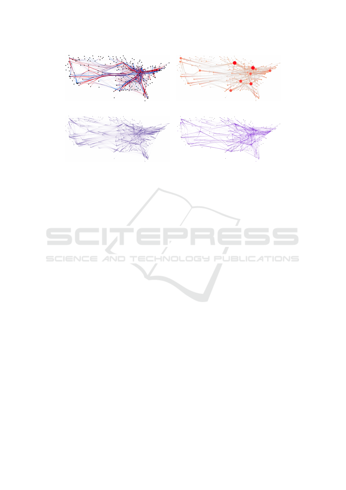
(a) Divided Edge Bundling

(b) Stub Bundling (Nocaj and Brandes, 2013)

(d) EEB with partial edges, α = 70

◦

Figure 5: Comparison of solutions for the USAirlines (G9).

and 77 single-bundled edges (318 bundles in total).

It is clear that the our group of bundles is markedly

different from the solutions generated by the Stub

Bundling and the SideKnot methods, since in our ap-

proach, they are formed respecting model constraints.

Overall, the experimental results suggest that the main

disadvantage of the EEB framework is its long run-

ning time for large graphs. As with most population-

based search algorithms, the running time for EEB

is inﬂuenced by the population size, the number of

generations, the size of the graph and other param-

eters. The evolutionary parameters were adjusted to

attempt to ﬁnd a near-optimal solution, which greatly

increased the running time.

Finally, the evolutionary edge bundling algorithm

attempted to satisfy, implicitly or explicitly, the aes-

thetics proposed in Section 4. For instance, the mini-

mization criteria of the total number of bundles, the

maximization of compatibility between edges, and

the maximization of the number of edges per bundle

are addressed by the objective function of CBEB (and

partially by ABEB) in EEB. Furthermore, bundling

only adjacent edges tends to minimize the ambiguity

of tracing edges. Symmetry was given by the use of

a force-directed edge bundling algorithm for render-

ing the results of EEB. The minimization of the total

number of crossings between edges and bundles was

addressed by using partial edge drawings.

10 CONCLUSIONS

This paper describes a new approach for edge

bundling by an approximate evolutionary algorithm

(EBB) in order to optimize edges to be grouped

into edge bundles. We examined angle-based edge

bundling which reduces angles between adjacent

edges, and compatibility-based edge bundling that

group edges with compatible directions and lengths.

A previously deﬁned combinatorial optimization

problem (ABEB) and a new problem (CBEB) are dis-

cussed and solved using the evolutionary method. As

far as we know, this is the ﬁrst evolutionary algo-

rithm for edge bundling modeled as a combinatorial

optimization problem. The method was implemented

and tested on a number of graphs, showing to be efﬁ-

cient at ﬁnding a near-optimal solution when the goal

is to create bundled graphs with the minimum num-

ber of bundles by joining only adjacent edges. This

work examined just two particular edge bundling op-

timization problems. Many other problems remain

open. Future research could focus on the expansion of

the approach to extend the ﬁtness function for multi-

objective search, in order to deal with new aesthet-

ics criteria. Investigating a complete rendering func-

tion that allows a more intrinsic way to route edges

and bundles, in order to produce smoother and more

readable drawings, may also be fruitful. Finally, con-

ducting some user-controlled studies may possibly es-

tablish if the EEB and new optimization-based edge-

bundling problems are visually appealing or effective

to help users to understand overall patterns.

ACKNOWLEDGEMENTS

This work has been supported by FAPEG-Brazil.

IVAPP 2018 - International Conference on Information Visualization Theory and Applications

142

REFERENCES

Alam, J., M.Fink, and Pupyrev, S. (2016). The bun-

dled crossing number. In 24th Internat. Symp. Graph

Drawing, pages 399–412.

Angelini, P., Bekos, M., Kaufmann, M., Kindermann, P.,

and Schneck, T. (2016). 1-fan-bundle-planar drawings

of graphs. In 24th Internat. Symp. Graph Drawing –

Poster, pages 634–636.

ack, T. (1996). Evolutionary Algorithms in Theory and

Practice: Evolution Strategies, Evolutionary Pro-

gramming, Genetic Algorithms. Oxford Univ. Press.

Battista, G., Eades, P., Tamassia, R., and Tollis, I. G. (1998).

Graph Drawing: Algorithms for the Visualization of

Graphs. Prentice Hall PTRr, 1st edition.

Bruckdorfer, T., Cornelsen, S., Gutwenger, C., Kaufmann,

M., Montecchiani, F., N

ollenburg, M., and Wolff, A.

(2012). Progress on partial edge drawings. CoRR,

abs/1209.0830.

Cui, W., Zhou, H., Qu, H., Wong, P., and Li, X. (2008).

Geometry-based edge clustering for graph visualiza-

tion. Trans. Vis. Comput. Graph, 14(6):1277–1284.

Ersoy, O., Hurter, C., Paulovich, F., Cantareiro, G., and

Telea, A. (2011). Skeleton-based edge bundling

for graph visualization. Trans. Vis. Comput. Graph,

12(17):2364–2373.

Ferreira, J. M., Nascimento, H. A. D., Quigley, A. J.,

and Foulds, L. R. (2017). Computational complex-

ity of edge bundling problemss. http://inf.ufg.

br/biblioteca-digital. Technical report, Federal

University of Goi

as.

Girvan, M. and Newman, M. (2002). Community struc-

ture in social and biological networks. Natl. Acad.

Sci. USA, 99(12):7821–7826.

Holten, D. (2006). Hierarchical edge bundles: Visualization

of adjacency relations in hierarchical data. Trans. Vis.

Comput. Graph, 12(5):741–748.

Holten, D. and van Wijk, J. (2009). Force-directed edge

bundling for graph visualization. Comput. Graph. Fo-

rum, 28(3):983–990.

Hurter, C., Ersoy, O., and Telea, A. (2012). Graph bundling

by kernel density estimation. Comput. Graph. Forum,

31(3):865–874.

ISGCI (2015). Information system on graph classes and

their inclusions. http://www.csun.edu/gd2015/

topics.htm. [Online; accessed 02-November-2017].

Knuth, D. (1993). The Stanford GraphBase: A Platform for

Combinatorial Computing. Addison-Wesley.

Lhuillier, A., Hurter, C., and Telea, A. (2017). State of the

art in edge and trail bundling techniques. Comput.

Graph. Forum, 36(3):619–645.

McKnight, R. L. (2015). Low-stretch trees for network vi-

sualization. Master dissertation, University of British

Columbia.

MovieLens (2017). Movielens. http://www.eecs.wsu.

edu/

yyao/. [Online; accessed 02-November-2017].

Newman, M. E. J. (2006). Modularity and community

structure in networks. National Academy of Sciences,

103(23):8577–8582.

Nguyen, Q. H., Hong, S., and Eades, P. (2011). Tgi-eb: A

new framework for edge bundling integrating topol-

ogy, geometry and importance. 19th Internat. Symp.

Graph Drawing, 7034:123–135.

Nocaj, A. and Brandes, U. (2013). Stub bundling and con-

ﬂuent spirals for geographic networks. In 21st Inter-

nat. Symp. Graph Drawing, pages 388–399.

Optimization, G. (2017). Gurobi optimizer quick start

guide. http://www.gurobi.com/documentation/.

[Online; accessed 14-May-2017].

Peng, D., N. Lu, W. C., and Peng, Q. (2012). Sideknot:

Revealing relation patterns for graph visualization. In

IEEE Paciﬁc Visualization Symposium, pages 65–72.

Pupyrev, S., Nachmanson, L., and Kaufmann, M. (2011).

Improving layered graph layouts with edge bundling.

In Internat. Symp. Graph Drawing, pages 329–340.

Saga, R. (2016). Quantitative evaluation for edge bundling

by difference of edge lengths and area occupation. In

HCI International Posters Extended Abstracts, pages

287–290.

Saroj, D. (2012). A non-revisiting genetic algorithm for op-

timizing numeric multi-dimensional functions. Intern.

Journal on Comput. Sciences and Applic., 2(1):83–93.

Selassie, D., Heller, B., and Heer, J. (2011). Divided edge

bundling for directional network data. Trans. Vis.

Comput. Graph, 17(12):2354–2363.

Skiena, S. (1990). Minimum Vertex Cover. § 5.6.2 in Imple-

menting Discrete Mathematics: Combinatorics and

Graph Theory with Mathematica. Addison-Wesley.

Zachary, W. (1977). An information ﬂow model for conﬂict

and ﬁssion in small groups. Journal of Anthropologi-

cal Research, 33(4):452–473.

An Evolutionary Algorithm for an Optimization Model of Edge Bundling

143