Slice-based Visualization of Brain Fiber Bundles

A LIC-based Approach

Stefan Philips

, Mario Hlawitschka

and Gerik Scheuermann

Leipzig University, Image and Signal Processing Group, Leipzig, Germany

Leipzig University of Applied Sciences, Faculty of Computer Science, Mathematics and Natural Sciences, Leipzig,

Germany

Keywords:

Fiber Bundles Visualization, Slice, MRI, dw-MRI, Tractography, Visualization, 2D.

Abstract:

The reconstruction of brain ﬁbers from diffusion MRI data is a widely studied ﬁeld. There is a great variety

of algorithms to generate ﬁber tracts. Despite the many possibilities to create ﬁber tractograms, it is not

very common within the medical community to make use of them. We think there are two reasons why the

acceptance of this technique is so low. The ﬁrst reason is that most time the degree of detail provided by

singular ﬁbers is neither justiﬁed nor needed. Second, within the medical domain tractography visualization

is still uncommon. To solve the ﬁrst problem it is common to apply clustering algorithms which aggregate the

single ﬁbers to ﬁber bundles. In this paper, we display the ﬁber bundles within slices. The presentation within

slices is common within the medical community and very intuitive to examine. Furthermore, our visualization

allows the spatial assignment of ﬁber bundles to the brain structure provided as T1 images. Among many

neuroscientists and physicians, T1 images are the main source for spatial orientation within the brain.

1 INTRODUCTION

Diffusion-weighted magnetic resonance imaging

(dw-MRI) is the only data source to reconstruct the

neuronal connections of a living brain. A dw-MR

image stores for each voxel the hydrogen diffusion

proﬁle. Brain ﬁbers/axons are ensheathed by myelin,

which is about 40 % water. Therefore the orientations

of the axons inﬂuence the hydrogen diffusion proﬁles.

Hence, it is possible to reconstruct nerve ﬁbers from

dw-MR images with tractography algorithms.

The dw-MR images are differentiated by their an-

gular resolution. The most commonly used diffusion

tensor images (DTI) with at least six measurements in

different directions allows it to derive one main diffu-

sion direction. The use of high angular resolution data

imaging (HARDI) with more measurements in, e.g.

60, different directions makes it possible to compute

a more realistic and detailed model of the diffusion

proﬁle per voxel. With the help of HARDI it is pos-

sible to extract several prominent diffusion directions

per voxel.

The diffusion characteristic can be described by

the diffusion orientation distribution function (ODF).

The diffusion ODF is the marginal probability of dif-

fusion in a given direction, which is computed for

each voxel. Tuch 2004 introduced the diffusion ODF

for dw-MRI. For our method, we use the improved

variant of Aganj et al. 2010.

For a better comprehension of the remaining text

we deﬁne the terms brain ﬁber, ﬁber and ﬁber bundle:

Brain Fiber: the actual biological

Fiber: a trajectory reconstructed from the dw-MR

data using a tractography algorithm

Fiber Bundle: a set of anatomically similar ﬁbers

Especially the differentiation between a brain

ﬁber and a ﬁber, which is reconstructed, is impor-

tant. One has to be aware that a 7 T Scanner has a

maximal voxel resolution of 1 mm edge length and

a typical axon has a diameter of 1 µm. Consider-

ing this, ten thousands of axons can run through one

voxel. With this in mind, one has to think of a recon-

structed ﬁber as a representative for many real brain

ﬁbers. Since a reconstructed ﬁber is already a sim-

pliﬁcation, it makes sense for many use cases sense

to reduce the data even more. This leads to the next

logical step: the clustering of the reconstructed ﬁbers

by similarity. This clustering is done by ﬁber bun-

dle algorithms, which typically use geometric shape

and position of the ﬁbers to measure similarity. The

similarity, in turn, is used to group the ﬁbers. These

groups are the ﬁber bundles.

Philips, S., Hlawitschka, M. and Scheuermann, G.

Slice-based Visualization of Brain Fiber Bundles - A LIC-based Approach.

DOI: 10.5220/0006619402810288

In Proceedings of the 13th International Joint Conference on Computer Vision, Imaging and Computer Graphics Theory and Applications (VISIGRAPP 2018) - Volume 3: IVAPP, pages

281-288

ISBN: 978-989-758-289-9

281

The awareness of the structural brain connectivity

should be very helpful for clinical and scientiﬁc ap-

pliances as well. But despite the ﬁber tractography

algorithms are well explored, the acceptance within

the medical community, especially in the clinical en-

vironment, is low.

(Hlawitschka et al., 2013) mentions the feedback

from neuroscience experts for slice-based methods is

very positive. The preference for slice-based visual-

izations among these experts has the following rea-

sons:

• A simple but undeniable fact is the familiarity

of neuroscientists and physicians with the slice-

based data presentation. Slices allow them to ex-

plore and focus the data in a familiar way.

• Especially during the exploration of brain related

data, the anatomical context is a very important

asset. This can be achieved by combining a sparse

slice visualization with anatomical image slices,

e.g. T1 images.

• Slice-based techniques avoid occlusions.

• Medical documentation is often done in 2D.

Further Munzner 2014 gives a comprehensive

overview of possible disadvantages resulting from 3D

visualizations.

In this work, we introduce a visualization tech-

nique that has all the aforementioned advantages.

Furthermore, our visualization works for difﬁcult

ﬁber conﬁgurations, like kissing or crossing ﬁbers,

and it can be used in combination with 3D ﬁber vi-

sualizations.

2 RELATED WORK

Our visualization approach relies on two kinds of pre-

processing algorithms. It needs a ﬁber tracking and a

ﬁber clustering algorithm.

There are a multitude of different ﬁber tracking

algorithms. Behrens et al. 2014 give an overview of

all three types of tractography algorithms. (Fillard

et al., 2011) benchmarks different approaches. Prob-

abilistic tractography algorithms are a special type of

ﬁber tracking algorithm, which do not generate 3D

trajectories as ﬁbers. Brieﬂy explained: Probabilistic

tractography algorithms compute for each voxel of a

dataset the connection likeliness to a seed voxels.

The trajectories of the aforementioned tractogra-

phy algorithms can be clustered by a ﬁber clustering

algorithm. Also for this task exists several algorithms.

The visualization of tractograms as 3D polylines

is a competing and complementing approach to our

technique as well. Therefore subsection 2.1 refers to

work that displays ﬁbers as 3D polylines.

In the last subsection, we present alternative slice-

based dMRI-related visualization techniques. This

overview of alternative techniques allows us to com-

pare our method to them.

2.1 Visualization of 3D Trajectories as

Polylines

The visualization of 3D trajectories has many appli-

cations and is therefore thematized by several pub-

lications which are not speciﬁcally related to recon-

structed brain ﬁbers, e.g. Zöckler et al. 1996 or Mallo

et al. 2005.

Eichelbaum et al. 2013 addressed the problem

of the spatial and the structural perception of recon-

structed brain ﬁbers to each other. With their LineAO

approach, they contributed an algorithm to display

ﬁbers with better spatial and structural perception.

2.2 Slice-based Visualization

Approaches

There already exist different approaches to visualize

reconstructed brain ﬁber data in a slice based manner.

Goldau et al. 2011 introduced a technique to vi-

sualize probabilistic tractograms slice-wise. This ap-

proach was improved regarding the perception of

tract probability by Hlawitschka et al. 2013. Lately

Reichenbach et al. 2015b adapted the approach to

HARDI data, that means they were able to illus-

trate possible kissing or crossing tracts of probabilis-

tic tractograms.

Höller et al. 2012 proposed a slice-based tech-

nique which is based on a three-dimensional LIC. The

necessary directions for the LIC is gained by extract-

ing up to two maxima from the diffusion ODFs. The

directions of the corresponding ﬁrst maxima are used

to apply a color coding to the LIC results. Höller et

al. 2014 modify their slice visualization approach by

replacing the input noise for the LIC algorithm with

an image of diffusion glyphs.

Calamante et al. 2011 introduced track-density

imaging (TDI). This technique counts the ﬁbers cross-

ing each voxel of a high resolution grid, allowing

more insight into the white matter structure. Color

coding can visualize the diffusion direction.

3 METHOD

In this section we introduce our slice-wise visualiza-

tion of ﬁber bundles. In combination with a T1 image

IVAPP 2018 - International Conference on Information Visualization Theory and Applications

282

as an anatomical context, this allows a clear assign-

ment of ﬁber bundles to the brain anatomy. These

ﬁber bundles shall be distinguishable and traceable

within the slice. We start by explaining the necessary

preprocessing steps – ﬁber tracking and ﬁber cluster-

ing. After that, we provide the detailed steps of our

approach to achieve the aforementioned visualization.

This includes:

• the creation of direction images for each bundle

• the creation of a noise texture, that allows the

blending of the ﬁber bundle LIC-images

• the blending of the LIC-images

3.1 Preprocessing

The basic data input for our visualization method is a

diffusion MRI dataset. Based on this data, our visu-

alization method needs two preprocessing algorithms,

the ﬁber tractography algorithm, and an algorithm to

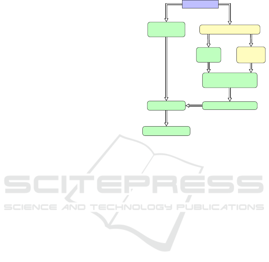
cluster the created ﬁbers by similarity. The depen-

dence of our processes is shown in Figure 1, where

the preprocessing algorithms are marked yellow.

For both steps, tracking and clustering exist a

bunch of algorithms. Behrens et al. 2014 give an

overview of tractography algorithms and the work by

Fillard et al. 2011 compares several ﬁber tracking al-

gorithms. (Reichenbach et al., 2015a) compare their

ﬁber clustering approach to four other techniques.

The preprocessing for our visualization starts with

a given diffusion MRI dataset. This is used to cre-

ate a ﬁber tractogram with a tracking algorithm. This

tractogram is then clustered by a ﬁber clustering ap-

proach. The preprocessing data-ﬂow is illustrated in

Figure 1.

3.2 Processing

Once the preprocessing is done, three types of data

are available for our visualization method. These are

the dMRI dataset, the tractography and the clustering

of the ﬁbers. The process ﬂow can be seen in Fig-

ure 1, where the actual visualization processes of our

method are marked green.

The overall bundle-slice creation process of the

bundle slices can be outlined the following four steps:

1. Create 2D direction images

(a) Voxelize Fibers:

calculate for each ﬁber which voxels it crosses

(b) Median bundle direction for each voxel:

calculate for each voxel the median direction

from all ﬁber of a bundle

create for each bundle per voxel the direction

dMRI dataset

Tractography algorithm

Voxelize

Fibers

Fiber

Clustering

Median bundle direc-

tion for each voxel

Extract 2D directions

Create Glyph

Noise Texture

LIC algorithm

Blend LIC images

Figure 1: Data-ﬂow during the processing. The colors pur-

ple, yellow or green mark if the boxes represent data, pre-

processing or processing steps, respectively.

2. Create Glyph Noise Texture:

create a noise texture for the LIC algorithm using

HARDI glyphs

3. LIC algorithm:

compute a LIC image for each ﬁber bundle of the

slice by using the 2D directions images from step

1 and the noise image from step 2

4. Blend LIC images:

combine the different LIC images into one image

3.2.1 Create 2D Directions Image

Voxelize Fibers

input: ﬁber tractography, ﬁber clustering

output: voxels with directions with annotated ﬁber

cluster number

We calculate for each ﬁber which voxel it passes and

store in each crossed voxel the local ﬁber direction.

Currently, the resolution of the voxelized ﬁbers is de-

termined by the input dMRI dataset.

In detail the voxelization algorithm works as fol-

low: The algorithm walks along the ﬁber points and

processes two consecutive points after another. To

determine which voxels are crossed by a ﬁber seg-

ment between two consecutive points p

and p

, we

use the rasterization algorithm Glassner (1990) which

is based on the Bresenham algorithm 1965. The seg-

ment direction, annotated with the ﬁber cluster num-

ber of the currently processed ﬁber, is stored in every

Slice-based Visualization of Brain Fiber Bundles - A LIC-based Approach

283

voxel that is determined by the aforementioned raster-

ization algorithm.

The result of this process are sets of directions

, B

, . . . in each voxel. These sets group the di-

rections, which are derived from the ﬁbers, to the dif-

ferent ﬁber bundles.

Bundle Median Direction for Each Voxel

input: voxels with directions with annotated ﬁber

cluster number

output: representative 3D direction for each ﬁber

bundle for each crossed voxel

Now that we have the sets of directions B

, B

, . . .

in each voxel with B

= {d

, d

, . . .}, we need to

derive one representative direction for each set. Let

be one of these sets. We ﬁnd the spatial median di-

rection d

i,med

∈ B

according to the following formula

i,med

= argmin

d∈B

∑

j=1

^(d

i j

, d), (1)

where ^(a, b) is the angle between the directions a

and b.

Extract 2D Directions

input: representative 3D direction for each ﬁber bun-

dle for each crossed voxel

output: 2D vector images for each visualized bundle

For each ﬁber bundle, that crosses the current slice, a

2D vector image needs to be created. We obtain the

2D direction d

of the ﬁber bundle i by mapping the

3D direction d

∈ B

to the slice plane. Given that our

slices are aligned to the XY-, XZ- or YZ-plane, this

can be done by taking the respective values of the 3D

vector. For example the 3D direction d

= (x, y, z)

mapped to the XY-plane leads to d

= (x, y)

3.2.2 Noise Image

The original LIC algorithm was proposed by Cabral

and Leedom 1993 and uses two images as input: a

2D vector image and a noise image. The creation of

the 2D vector image is described in the previous para-

graph. Usually an image with white noise is as an

input for the LIC-algorithm.

Glyph-based Noise Image

input: dMRI dataset

output: 2D gray scale image with glyphs

Höller et al. 2014 use samples of ﬁber-orientation-

density (FOD) glyphs to generate a noise image for

the LIC. The ﬁber orientations for the FOD glyphs are

computed by using spherical deconvolution (Tournier

et al., 2004) on the HARDI input. Then the glyph

samples are placed along a path which results from a

deterministic tracking within the slice.

For our visualization we use like Höller et al. 2014

a from glyphs generated noise image. For our goal to

display clustered ﬁbers within slices, we cannot use

this a deterministic tracking algorithm. The determin-

istic tracking would most likely differ from the ﬁbers

to display and would be computational expensive.

Therefore we had to ﬁnd a good placement

scheme for the glyphs within the noise image. At a

ﬁrst glance the well-known glyph packing strategy by

Kindlmann and Westin 2006 seems a suitable choice

for the glyph placement problem, but it is designed

for DTI Glyphs and would have to be extended for

HARDI glyphs. Even if an extended variant would

be available, it would be unnecessary complex for the

actual task. In our case, the potential overlapping of

some glyphs within the noise image is not problem-

atic at all.

We tested three glyph placement strategies. The

ﬁrst one is a simple two-dimensional regular place-

ment. The second variant distributes the glyphs uni-

form randomly within the slice. And the third variant

uses Poisson-disk distribution to distribute the glyphs

within the slice.

Points of a Poisson-disk distribution are ran-

domly distributed and must be no closer than a spec-

iﬁed value. To create this distribution we used

the sampling algorithm proposed by Dunbar and

Humphreys 2006. Our concrete implementation com-

putes points within the 2D-range of [0..1] × [0..1].

These coordinates are scaled to the full image size.

Figure 2 shows examples for the different glyph

distributions. In Figure 2a one can see that the regu-

lar distribution pattern causes a regular pattern in the

result image. The uniform random distribution causes

a wild pattern in the resulting image, Figure 2b. The

Poisson-disk distribution results in straight lines, Fig-

ure 2c.

The actual glyphs are created as follows: A icosa-

hedron is tessellated with triangles to a certain degree.

Then the normalized triangle vertex coordinates are

used as input for the spherical harmonic function of

the ODF. The resulting values describe the surface of

the spherical function. This results in spherical har-

monics glyphs like shown in Figure 3. The tessel-

lation degree for these example glyphs is 2, which

means each consists of 162 vertices. The coloring is

done by using the absolute values of the normalized

IVAPP 2018 - International Conference on Information Visualization Theory and Applications

284

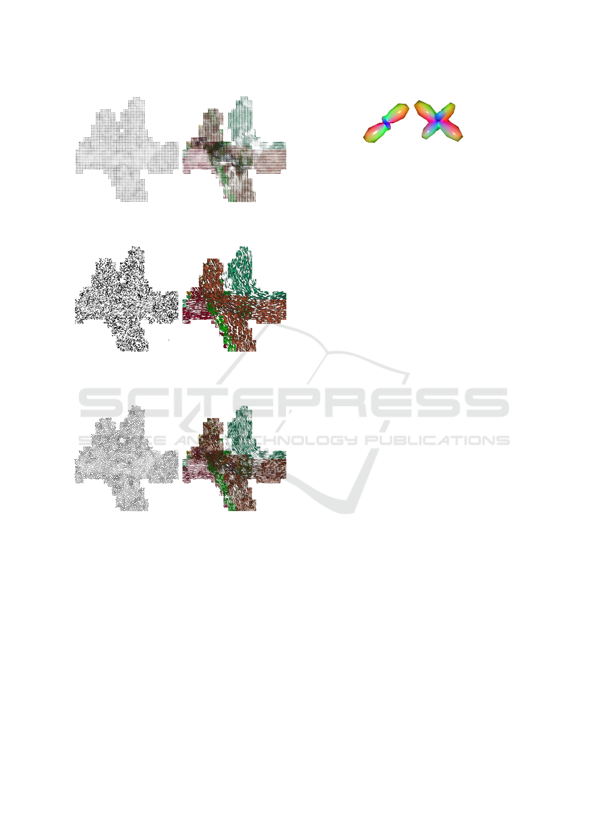
(a) Regular glyph distribution

Left: Noise image with regularly placed glyphs.

Right: The resulting visualization for regulary placed glyphs.

(b) Uniform random glyph distribution

Left: Noise image with uniform randomly placed glyphs.

Right: The resulting visualization for uniform randomly

placed glyphs.

Left: Noise image with Poisson-disk distributed glyphs.

Right: The resulting visualization for Poisson-disk dis-

tributed glyphs.

Figure 2: Different glyph distributions and the correspond-

ing result of the algorithm.

Euclidean direction as RGB color.

3.2.3 Special Case: Orthogonal Bundles

Fiber bundles which run orthogonal or almost orthog-

onal to the displayed slice would not be visualized in a

reasonable way by the LIC-method. This results from

the fact that there is not enough directional informa-

tion for this bundles within the slice.

Therefore we determine the orthogonal bundles

and display them by coloring their slice area with their

Figure 3: Spherical harmonics glyphs composited from 162

vertices. The absolute values of the Euclidean direction vec-

tors are used as RGB color vector (RGB coloring).

transparent cluster color (alpha value 0.5). Which

ﬁber bundles are considered to be orthogonal bundles

is determined by the percentage of the average bundle

direction-vector-component that is orthogonal to the

current slice.

3.2.4 LIC Process and Coloring

input: direction image for each bundle that crosses

the current slice and the glyph noise image

output: a LIC image for each bundle that crosses that

crosses the current slice

The LIC implementation is the original algorithm like

it was proposed by Cabral and Leedom 1993, but of

course it uses the adapted noise image. The coloring

is done bundle-wise, apart from that the actual color

of each ﬁber bundle can be arbitrary selected. For ex-

ample one can use RGB direction coloring, selection

coloring or any other bundle-wise coloring.

3.2.5 Blending the Bundle Layers

input: a LIC image for each bundle that crosses the

current slice

output: ﬁnal slice

After the LIC algorithm is done for every bundle. It

is necessary to merge the output of all LIC processes

into one image. This is done by drawing one LIC im-

age after another into the space left by the previous

LIC images. A pixel with RGB color c is considered

free if kck

max

< 0.2 is true. The blending order is de-

termined by the size of the bundles within the slice.

The blending process starts with the LIC image of

the smallest bundle. This should ensure the maximum

visibility of the ﬁber bundles in the slice.

4 RESULTS

We tested our visualization with two datasets. The

ﬁrst one is the synthetic Fiber Cup phantom dataset

(Fillard et al., 2011). The Fiber Cup dataset is a

dw-MRI scan of a hardware phantom. It was orig-

inally created to test tractography algorithms. We

Slice-based Visualization of Brain Fiber Bundles - A LIC-based Approach

285

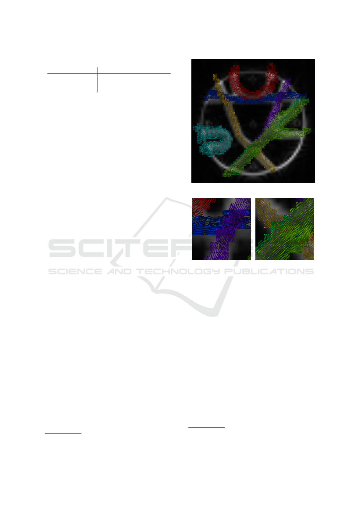
Table 1: Properties of the datasets to test the visualization.

Dataset Fiber Cup Human brain

voxel size (mm

) 3 × 3 × 3 1.7 × 1.7 × 1.7

dimensions 64 × 64 × 3 128 × 128 × 72

diffusion directions 128 60

choose this one because of its clear structure and the

known ground truth. It has typical difﬁcult ﬁber bun-

dle conﬁgurations like kissing, crossing and spread-

ing ﬁber bundles. The second one is a dw-MR im-

age of a healthy human brain. It was acquired with

a 3 T Siemens Trio MRI scanner using single echo

spin echo Echo-Planar Imaging (EPI) sequence with

GRAPPA on a 32 channel coil. Table 1 shows the

image properties of both datasets.

4.1 Fiber Cup Dataset

Figure 4a shows the whole dataset using our visual-

ization. The planar shape and the different ﬁber bun-

dle conﬁgurations make the Fiber Cup dataset ideal

to demonstrate slice based visualization approaches.

Since we know the ground truth of the Fiber Cup

dataset we reduced it by removing identiﬁed out-

liers to 250 ﬁbers. The ﬁbers were generated with

the streamline tractography algorithm by Lazar et

al. 2003 using the implementation from tensor toolkit

1.4

. Except for FA

= 0.2 and FA

= 0.3 we used

the default parameter. We used the QuickBundles

(Garyfallidis et al., 2012) algorithm to cluster the trac-

tograms. Heuristically we determined the parameter

θ = 225 to get a clustering close to the known ground

truth of 7 ﬁber bundles.

For the visualization example in Figure 4a we

used a Poisson-disk radius of 0.0045, a glyph size

of 0.4 and 30 LIC steps at maximum. The separate

ﬁber bundles are clearly identiﬁable and the course at

crossings is also traceable. The close-ups of cross-

ings in Figure 4b and 4c show that the bundles are

clearly differentiable The image shows also a disad-

vantage of the current implementation: Due to the low

resolution of the voxelized ﬁbers, the displayed ﬁber

bundles overlap the white matter. The low resolution

is also the reason for the raw block shape of the dis-

played ﬁbers.

4.2 Human Brain Dataset

The dataset of a healthy human brain allows us to

show a real world example. Figure 5a visualizes a

frontal view of a coronal slice. We used the determin-

istic spherical-deconvolution (SD) (Tournier et al.,

https://gforge.inria.fr/projects/ttk

(a) Visualization for the ﬁbercup dataset bundles.

(b) Detail of the crossing

in the upper-right area.

the bottom-middle area.

Figure 4: The presented algorithm applied to the Fiber Cup

dataset, including three detail views.

2004) based ﬁber tracking algorithm from MRtrix

with its default parameters. The clustering was done

with the approach by Reichenbach et al. 2015a. For

the visualization, we used the same parameter as be-

fore, a Poisson-disk radius of 0.0045, a glyph size of

0.4 and 30 LIC steps at maximum. We selected a slice

where the corticospinal tracts (CST, blue) and the cor-

pus callosum (CC, red) cross. The detail views of the

crossings in the left and right hemisphere are shown

in Figure 5c and 5b, respectively. The corticospinal

tract is traceable crossing the corpus callosum.

Figure 6 shows the LineAO approach by Eichel-

baum et al. 2013 and our slice-based visualization

combined. To select the displayed 3D trajectories,

we used a Region-of-Interest (ROI) box. By using

this combination, the user can beneﬁt from the advan-

tages of 2D and 3D visualization. Whereas the 3D

trajectories provide a good overview, the strength of

http://jdtournier.github.io/mrtrix-

0.2/tractography/tracking.html

IVAPP 2018 - International Conference on Information Visualization Theory and Applications

286

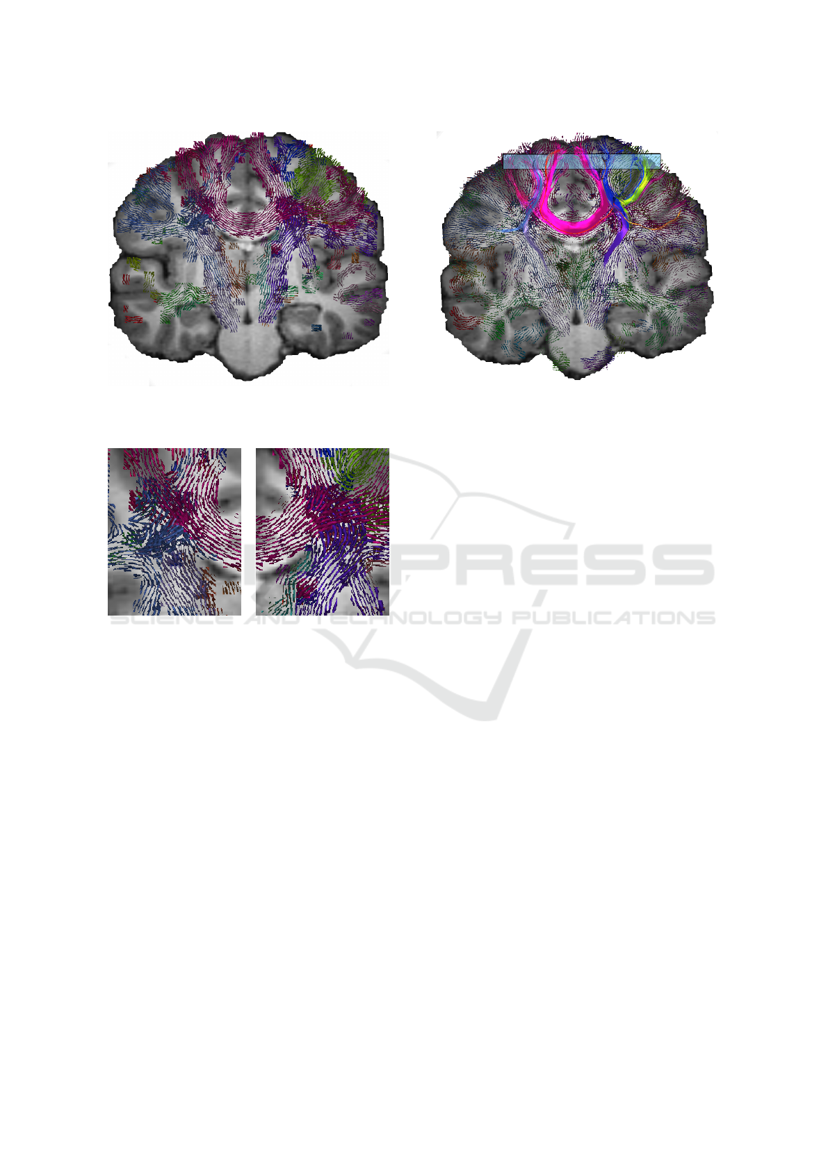
(a) Visualization for a coronal slice. Showing among

other ﬁber bundles the corpus callossum (CC, red) and

the cortico spinal tract (CST, blue.)

(b) Crossing of CC (red)

and CST (blue) in the right

hemisphere.

and CST (blue) in the left

hemisphere.

Figure 5: Visualization of Coronal slice and two detail

views. Orthogonal ﬁber bundles are suppressed.

our approach is the fast view into spatial details, with-

out using a ROI box and the clear perception of the

anatomical context, represented as T1 image.

4.3 Comparison to Existing

Visualizations

Depending on the application the presented method

has advantages over the previously mentioned visual-

ization approaches.

In contrast to 3D polylines, a slice based ﬁber

bundle visualization allows the easy assignment to an

anatomical context by using T1 images. Besides the

slice-wise view to medical data is well-established.

Given that slice-based methods are two-dimensional,

they are suitable for clinical documentation purposes.

The advantage of the presented method over the

Figure 6: The combination of 3D streamline and slice-based

visualization.

approach by Höller et al. 2014 is the use of recon-

structed tractograms. Höller et al. 2014 perform an

own tracking for their visualization. This tracking is

reduced to the currently displayed slice. Because of

this locality, it does not cover the complex task of ﬁber

reconstruction from diffusion MRI data. The com-

parison of ﬁber tractography algorithms by Fillard et

al. 2011 suggests that especially the use of global in-

formation is advisable. The presented method can use

many available ﬁber tractography algorithms. The in-

formation complexity of the reconstructed ﬁber con-

ﬁgurations is further decreased by the use of a ﬁber

bundle algorithm.

The method by Reichenbach et al. 2015b is spe-

cialized for probabilistic tractograms. The adaptation

to general ﬁber tractograms would be possible, but the

visualization of deterministic ﬁber tractograms in a

glyph-based manner is counter-intuitive and increases

unnecessarily the visual complexity.

The aforementioned TDI approach (Calamante

et al., 2011) generates a super-resolution T1-like im-

age from a tractogram. TDI does not aim to visualize

concrete ﬁbers or ﬁber bundles.

5 SUMMARY

We presented a new visualization approach that al-

lows a slice-wise examination of ﬁber bundles. This

slice-wise inspection has several useful properties and

is intended as a supplement to conventional 3D trajec-

tory visualization of ﬁber bundles. The combination

of this visualization techniques is shown in Figure 6.

Further, the slice-wise presentation allows a clear

assignment of the ﬁber bundles to the structural infor-

Slice-based Visualization of Brain Fiber Bundles - A LIC-based Approach

287

mation provided by a T1 image. Many neuroscien-

tists use the structural information provided by a T1

image as spatial orientation. The familiarity of medi-

cal staff with slice-based data can also be considered

as an advantage of the method. Furthermore, a 2D vi-

sualization is well suited for medical documentation.

Another inherent advantage of a 2D approach is the

avoidance of occlusion.

We have shown that the visualization works also

for difﬁcult ﬁber bundle conﬁgurations like crossings,

see the Figures 5b, 5c, 4b, and 4c. The visibility of

the relation between the ﬁber bundles and anatomy

is a strength of the visualization method, too. The

Figures 4a and 5a allow it to relate the ﬁber bundle to

structural information given by T1 image.

REFERENCES

Aganj, I., Lenglet, C., Sapiro, G., Yacoub, E., Ugurbil, K.

and Harel, N. (2010). Reconstruction of the orientation

distribution function in single-and multiple-shell q-ball

imaging within constant solid angle. Magnetic Reso-

nance in Medicine 64, 554–566.

Behrens, T. E., Sotiropoulos, S. N. and Jbabdi, S. (2014).

MR Diffusion Tractography. In Diffusion MRI - Sec-

ond Edition, (Johansen-Berg, H. and Behrens, T. E., eds),

chapter 19, pp. 429–451. Elsevier Inc. London.

Bresenham, J. E. (1965). Algorithm for computer control

of a digital plotter. IBM Systems journal 4, 25–30.

Cabral, B. and Leedom, L. C. (1993). Imaging Vector

Fields Using Line Integral Convolution. In Proceed-

ings of the 20th Annual Conference on Computer Graph-

ics and Interactive Techniques SIGGRAPH ’93 pp. 263–

270, ACM, New York, NY, USA.

Calamante, F., Tournier, J.-D., Heidemann, R. M., Anwan-

der, A., Jackson, G. D. and Connelly, A. (2011). Track

density imaging (TDI): validation of super resolution

property. Neuroimage 56, 1259–1266.

Dunbar, D. and Humphreys, G. (2006). A Spatial Data

Structure for Fast Poisson-disk Sample Generation. In

ACM SIGGRAPH 2006 Papers SIGGRAPH ’06 pp.

503–508, ACM, New York, NY, USA.

Eichelbaum, S., Hlawitschka, M. and Scheuermann, G.

(2013). LineAO — Improved Three-Dimensional Line

Rendering. IEEE TVCG 19, 433–445.

Fillard, P., Descoteaux, M., Goh, A., Gouttard, S., Jeuris-

sen, B., Malcolm, J., Ramirez-Manzanares, A., Reisert,

M., Sakaie, K., Tensaouti, F., Yo, T., Mangin, J.-F. and

Poupon, C. (2011). Quantitative evaluation of 10 tractog-

raphy algorithms on a realistic diffusion MR phantom.

NeuroImage 56, 220 – 234.

Garyfallidis, E., Brett, M., Correia, M. M., Williams, G. B.

and Nimmo-Smith, I. (2012). Quickbundles, a method

for tractography simpliﬁcation. Frontiers in neuroscience

6, 175.

Glassner, A. (1990). Graphics Gems I.

Goldau, M., Wiebel, A., Gorbach, N. S., Melzer, C.,

Hlawitschka, M., Scheuermann, G. and Tittgemeyer, M.

(2011). Fiber Stippling: An Illustrative Rendering for

Probabilistic Diffusion Tractography. In IEEE BioVis

Proceedings pp. 23–30, IEEE.

Hlawitschka, M., Goldau, M., Wiebel, A., Heine, C. and

Scheuermann, G. (2013). Hierarchical Poisson-Disk

Sampling for Fiber Stipples. In 3rd Intl. Workshop on

VMLS pp. 19–23, Eurographics, Leipzig.

Höller, M., Otto, K. M., Klose, U., Groeschel, S. and

Ehricke, H. H. (2014). Fiber Visualization with LIC

Maps Using Multidirectional Anisotropic Glyph Sam-

ples. Journal of Biomedical Imaging 2014, 9:9–9:9.

Höller, M., Thiel, F., Otto, K.-M., Klose, U., Ehricke,

H.-H. and Schwedenschnaze, Z. (2012). Visualization

of High Angular Resolution Diffusion MRI Data with

Color-Coded LIC-Maps. In GI-Jahrestagung pp. 1112–

1124, GI.

Kindlmann, G. and Westin, C.-F. (2006). Diffusion tensor

visualization with glyph packing. IEEE Transactions on

Visualization and Computer Graphics 12.

Lazar, M., Weinstein, D. M., Tsuruda, J. S., Hasan, K. M.,

Arfanakis, K., Meyerand, M. E., Badie, B., Rowley,

H. A., Haughton, V., Field, A. et al. (2003). White matter

tractography using diffusion tensor deﬂection. Human

brain mapping 18, 306–321.

Mallo, O., Peikert, R., Sigg, C. and Sadlo, F. (2005). Illu-

minated lines revisited. In VIS 05. IEEE Visualization,

2005. pp. 19–26, IEEE.

Munzner, T. (2014). Visualization analysis and design.

CRC press.

Reichenbach, A., Goldau, M., Heine, C. and Hlawitschka,

M. (2015a). V-Bundles: Clustering Fiber Trajectories

from Diffusion MRI in Linear Time. In MICCAI (1),

(Navab, N., Hornegger, J., III, W. M. W. and Frangi,

A. F., eds), vol. 9349, of LNCS pp. 191–198, Springer.

Reichenbach, A., Goldau, M. and Hlawitschka, M. (2015b).

Fiber Stipples for Crossing Tracts in Probabilistic Trac-

tography. In Proc. of VCMB ’15 pp. 113–122, EG.

Tournier, J.-D., Calamante, F., Gadian, D. G. and Connelly,

A. (2004). Direct estimation of the ﬁber orientation den-

sity function from diffusion-weighted MRI data using

spherical deconvolution. NeuroImage 23, 1176–1185.

Tuch, D. S. (2004). Q-ball imaging. Magnetic resonance in

medicine 52, 1358–1372.

Zockler, M., Stalling, D. and Hege, H.-C. (1996). Interac-

tive visualization of 3D-vector ﬁelds using illuminated

stream lines. In Visualization’96. Proc. pp. 107–113,

IEEE.

IVAPP 2018 - International Conference on Information Visualization Theory and Applications

288