
3D Orientation Estimation of Industrial Parts from 2D Images using
Neural Networks
Julien Langlois
1,2
, Harold Mouchère
1
, Nicolas Normand
1
and Christian Viard-Gaudin
1
1
University of Nantes, Laboratoire des Sciences du Numérique de Nantes, UMR 6004, France
2
Multitude-Technologies a company of Wedo, France
Keywords:
Neural Networks, 3D Pose Estimation, 2D Images, Deep Learning, Quaternions, Geodesic Loss, Rendered
Data, Data Augmentation.
Abstract:
In this paper we propose a pose regression method employing a convolutional neural network (CNN) fed with
single 2D images to estimate the 3D orientation of a specific industrial part. The network training dataset
is generated by rendering pose-views from a textured CAD model to compensate for the lack of real images
and their associated position label. Using several lighting conditions and material reflectances increases the
robustness of the prediction and allows to anticipate challenging industrial situations. We show that using a
geodesic loss function, the network is able to estimate a rendered view pose with a 5
◦
accuracy while inferring
from real images gives visually convincing results suitable for any pose refinement processes.
1 INTRODUCTION
Pose estimation of objects has recently gained lots of
interest in the literature for its wide application possi-
bilities such as robotic grasping for bin picking. Nev-
ertheless, this task remains challenging in the case of
industrial parts, usually texture-less and not appropri-
ate for key-points and local descriptors. Moreover,
in a non-controlled and unfriendly industrial environ-
ment many issues have to be tackled akin to low lu-
minosity or cluttered scenes. To be embedded in a bin
picking process, any pose estimation module requires
high precision recognition while offering acceptable
execution speed not to penalize the following indus-
trial treatments. It is even more arduous when the part
needs to be precisely placed on an assembly module
afterwards.
Estimating the position of any 3D objects in a scene
has gained interest in the past years thanks to neural
networks and their abilities to extract relevant features
for a given task. However, this task remains challeng-
ing when handling industrial parts because of their of-
ten black and glossy plastic material: in hostile plant
conditions this material is known to constrain the pre-
diction capabilities of image-based algorithms.
Many works have been conducted with a depth infor-
mation allowing algorithms to learn spatial features to
recognize (Bo et al., 2012) or estimate the positions of
objects within an image (Hodan et al., 2015) (Shot-
ton et al., 2013). In this paper we show that a simple
2D information is enough to predict the rotations of a
part given a certain confidence score using a CNN and
quaternions. However, the training dataset creation
based on real images appears to be a painful process.
Thereby, we also propose a dataset generation frame-
work using rendered views from a CAD (Computer-
Aided Design) model as a way to offset the lack of
real images labeled with the accurate object position
(Su et al., 2015). Using an alpha channel (trans-
parency) offers the possibility to add backgrounds and
rotations without any image cropping. Scene param-
eters (lightening, scale, reflectance...) must be deci-
sive for a relevant feature learning to infer from real
images thus we choose them according to the part ap-
pearances in real views (Mitash et al., 2017).
When directly regressing the pose of an object, the
Euclidean distance is often employed as a loss func-
tion to approximate the distance between quater-
nions (Melekhov et al., 2017) (Kendall et al., 2015)
(Doumanoglou et al., 2016). In this paper we pro-
pose a geodesic distance-based loss function using
the quaternion properties. Operations of the quater-
nion algebra are a combination of simple derivable
operators which can be used in a gradient-based back-
propagation. We achieve to get a network which of-
fers a great pose estimation with a low uncertainty
over the data. With a wide variety of scene param-
eters, the network is able to estimate the pose of the
Langlois, J., Mouchère, H., Normand, N. and Viard-Gaudin, C.
3D Orientation Estimation of Industrial Parts from 2D Images using Neural Networks.
DOI: 10.5220/0006597604090416
In Proceedings of the 7th International Conference on Pattern Recognition Applications and Methods (ICPRAM 2018), pages 409-416
ISBN: 978-989-758-276-9
Copyright © 2018 by SCITEPRESS – Science and Technology Publications, Lda. All rights reserved
409

object in a real image with a sufficient accuracy to be
fed into a pose refinement process.
2 RELATED WORK
2.1 Local Features Matching
Local features extraction has been widely studied in
the literature as it easily gives matching pair opportu-
nities between two views. These features were first
constructed from parametric shapes isolated within
the image contours (Honda et al., 1995). The indus-
trial parts need to have specific shape singularities
to be properly localized, though. More recently, the
well known SIFT local descriptor was employed to
get a pose description of an object (Lowe, 2004). In
(Gordon and Lowe, 2004) a matching between the ex-
tracted SIFT with the pose description of the object
is performed to get a camera pose estimation. Be-
cause of the high dimension of the features vector,
the S IFT severely impacts the algorithm computa-
tion time. Later, the SURF local descriptors, faster
to extract, were introduced. However, they appear to
be less robust to rotation and image distorsion than
SIFT (Bay et al., 2008). To be computed, the local
descriptors often rely on the object texture, one el-
ement absent from industrial parts. Moreover, they
suffer from high luminosity and contrast variations
which make them improper to be used in a challeng-
ing plant environment. Using the depth channel of
RGB-D images, (Lee et al., 2016) proposes an ICP al-
gorithm fed with 3D SURF features and Closed Loop
Boundaries (CLB) to estimate the pose of industrial
objects. However, the system can not deal with oc-
clusions likely to happen inside a bin.
2.2 Template Matching
To tackle the issue of texture-less objects, template
matching methods are employed to assign more com-
plex feature pairs from two different points of view.
Prime works built an object descriptor composed of
different templates hierarchically extracted from an
object point of view and later compared with an input
image through a distance transform (Gavrila, 1998).
To handle more degrees of freedom in the camera
pose estimation, the recent machine learning tech-
niques are used to learn the object templates and
the associated camera pose to infer the position and
then refine it using the distance transform. However,
the algorithms still need a contour extraction pro-
cess which is not suitable for low contrasted, noisy
or blurred images. In (Hinterstoisser et al., 2010) the
discretized gradient directions are used to build tem-
plates compared with an object model through an en-
ergy function robust to small distorsion and rotation.
This method called LINE is yet not suitable for clut-
tered background as it severely impacts the computed
gradient. A similar technique is proposed in (Muja
et al., 2011). The arrival of low-cost RGB-D cameras
led the templates to become multimodal. LINEMOD
presented in (Hinterstoisser et al., 2011) uses a depth
canal in the object template among the gradient from
LINE to easily remove background side effects. The
method is later integrated into Hough forests to im-
prove the occlusion robustness (Tejani et al., 2014).
To deal with more objects inside the database, (Hodan
et al., 2015) proposes a sliding window algorithm ex-
tracting relevant image areas to build candidate tem-
plates. These templates are verified to get a rough
3D pose estimation later refined with a stochastic op-
timization procedure. The camera pose estimation
problem can be solved with template matching but re-
mains constrained to RGB-D information to achieve
acceptable results. In this paper we propose to use 2D
images without depth information therefore not suit-
able for this type of matching.
2.3 Features Matching from Neural
Networks
Neural networks offer the ability to automatically ex-
tract relevant features to perform a given task. In
a pose estimation problem they use convolutional
neural networks to compute object descriptors as a
database prior to a kNN algorithm to find the closest
camera pose in the set (Wohlhart and Lepetit, 2015).
The loss function is fed with a triplet formed with
one sample from the training dataset and two others
respectively close and far from the considered cam-
era position. Forcing the similarity between features
and estimated poses for two close points of view is
also employed in (Doumanoglou et al., 2016) with a
Siamese neural network doing a real pose regression.
Although these methods are quite appealing, they still
take advantage of RGB-D modalities. In (Kendall
et al., 2015) a deep CNN known as PoseNet based
on the GoogLeNet network is built to regress a 6D
camera pose from a 2D image. Whereas slightly dif-
ferent from our work for dealing with urban scenes,
the work shows the continuous 3D space regression
capability of a CNN in an end-to-end manner. Other
works are using pre-trained CNN for object classifi-
cation to estimate a view pose through SVMs. The
depth channel of the RGB-D image is converted into
an RGB image to be fed into a CNN with relevant 3D
features (Schwarz et al., 2015).
ICPRAM 2018 - 7th International Conference on Pattern Recognition Applications and Methods
410
3 POSE REGRESSION
In this section we first define and transform the pose
regression problem as a camera pose estimation prob-
lem using a bounding sphere and quaternions. To gen-
erate the pose views later fed into the CNN, a 3D
pipeline rendering a CAD model seen under several
scene atmosphere conditions is presented. Finally,
the convolutional neural network which regresses the
pose of the object is described from its architecture to
its loss function based on the geodesic distance in the
quaternions space.
3.1 Problem Definition
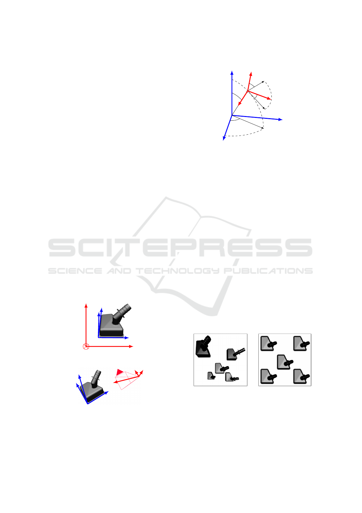
An object O is placed in a world scene with its frame
position P
O
= (x
O
,y
O
,z
O
) and orientation expressed
as the Euler triplet R
O
= (φ
O
,θ
O
,ψ
O
). The objec-
tive is to retrieve the object orientation from a point
of view given by a fixed top camera. A trivial prob-
lem shift is to consider a fixed object with a mo-
bile camera encompassing the scene localized with
R
C
= (φ
C
,θ
C
,ψ
C
) lying on a bounding r-radius sphere
centered on the object’s centroid (Figure 1). Using
the convention Z −Y − Z for the Euler triplet allows
us to easily map the camera position according to the
sphere azimuth and elevation. The third angle ψ
C
is
then the camera plane rotation angle (Figure 2).
Any composition of rotations can be written as
an axis-angle rotation according to the Euler’s rota-
tion theorem. Following this equivalence, to avoid
any gimbal locks and improve computation perfor-
mances, the triplet R
C
is written as the quaternion
~
X
O
~
Z
O
~
Y
O
~
Y
C
~
X
C
~
Z
C
~
X
O
~
Z
O
~
Y
O
~
Y
C
~
Z
C
~
X
C
Figure 1: Top: The object O placed in the world scene and
its CAD frame (
~
X
O
,
~
Y
O
,
~
Z
O
) viewed from a fixed top-view
camera. Bottom: Finding the O frame is equivalent to a
camera frame (
~
X
C
,
~
Y
C
,
~
Z
C
) evaluation problem in the scene
when the object is fixed.
~
X
O
~
Y
O
~
Z
O
φ
C
θ
C
~
Z
C
~
Y
C
~
X
C
ψ
C
ψ
C
Figure 2: The camera is placed according to the
(φ
C
,θ
C
,ψ
C
) Euler’s triplet using the Z −Y − Z convention.
q
C
= (w
C
, ~v
C
) according to the chosen Euler conven-
tion, representing an axis-angle rotation with a vector
expressed as an hypercomplex number. Any camera
orientation is now independent from the Euler’s con-
vention used.
Using a telecentric lens on the camera would allow
us to estimate the position P
O
and orientation R
O
of a
part without any perspective effect: two objects sim-
ilarly orientated but widely separated in the world
scene would take the same shape in the top-view cam-
era plane. The side effect is that different Z altitudes
would give identical zooms (subject to magnifying er-
rors) thus misleading the frame position estimation
(Figure 3). It means that the system still needs to
use an entocentric lens to predict the r sphere radius.
Knowing the object centroid in the image plan plus
the estimated r sphere radius is enough to obtain each
object frame position P
O
among R
C
from our neural
network prediction. The position estimation P
O
re-
mains out of this paper scope yet so we suppose the
radius r is known and we only use entocentric render-
ing for the orientation estimation R
C
.
Figure 3: Same scene rendered with different camera lens.
Left: entocentric lens rendering different altitude and per-
spectives. Right: telecentric lens giving the same aspect for
every object including scale.
3D Orientation Estimation of Industrial Parts from 2D Images using Neural Networks
411
3.2 Pose Generation
The industrial parts inside a bin have many possible
poses as they can lie on each other. Thereby, creating
a training dataset of real images covering all possibil-
ities is tedious and complex. Moreover, every point
of view will rely on a specific lightening condition
not necessarily consistent with different bin-picking
module placements in a factory. In this work a CAD
model of the object is available so that a dataset can be
generated during a rendering process. Using a virtual
dataset has several advantages including the anticipa-
tion of different atmosphere conditions, backgrounds,
scene cluttering and occlusions happening in a non-
favorable plant environment.
3.2.1 Camera Placement
A CAD model is placed on the center of a 3D scene
according to its frame then textured to reproduce the
glossy black plastic material of the real part. The
camera positions are evenly picked on an r radius
sphere surface with a specified number of poses us-
ing a golden spiral algorithm (Boucher, 2006). The
camera frame is computed so that the
~
Z axis is point-
ing toward the scene center and the
~
X axis remains
horizontal (meaning ψ
C
= 0). This results in two an-
gles φ
C
and θ
C
positioning and a camera plane rota-
tion ψ
C
. Notice that this third angle can be generated
by rotating the result image which can be done on the
fly during the training phase thus reducing the dataset
size on the hard drive.
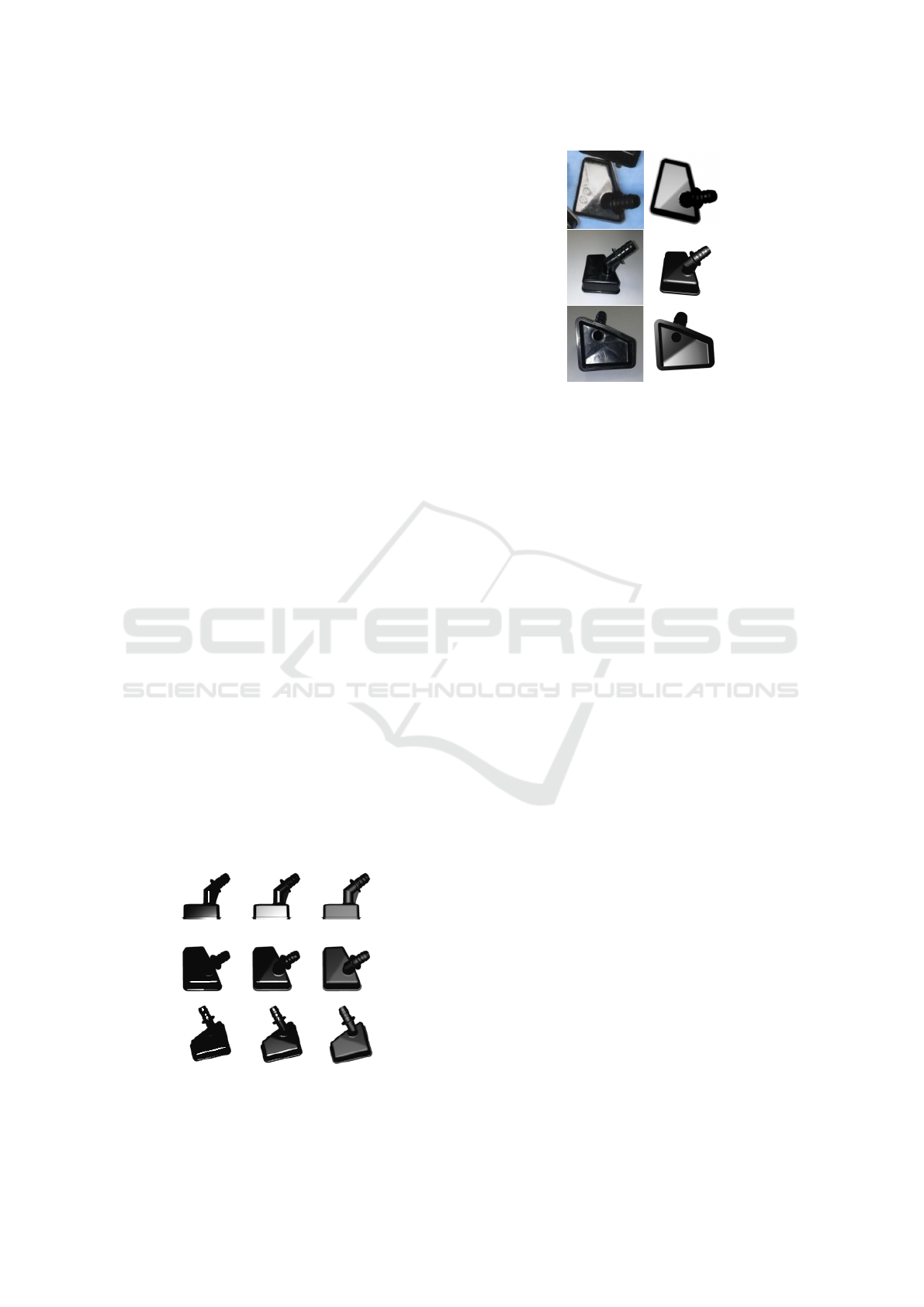
3.2.2 Scene Parameters
For each point of view, the lighting conditions as well
as the material reflectance are modified. This em-
phasizes different areas of the part so that the neural
network can learn different features from the training
dataset (Figure 4). A relevant scene parameter range
Figure 4: Effects of several lightening conditions in the
scene and different object material reflectances on the ren-
dered image.
Figure 5: Relevant scene parameters can render realistic
views of the part. Left: the real image pose. Right: the
rendered approximated pose.
comes from the study of real images taken under sev-
eral conditions as shown in Figure 5. However, this
might not always look realistic since the real material
has no constant reflectance on its surface and it may
contains blur or timestamp prints as seen in the top-
left image in Figure 5. Finally, to avoid any pixelation
the software antialiasing is applied and the image is
generated with a size of 64 × 64 pixels. This image
resolution is approximately the object bounding box
size inside a bin rendered with an initial camera res-
olution of 1600 × 1200 pixels (which is an industrial
standard) at a working distance of 2 meters.
The scene background is set as an alpha channel (full
transparency) to apply different backgrounds on the
fly during the future training phase (Figure 8). The
background can be defined as a color or a texture
picked within high resolution samples showing mate-
rial such as wood, plastic or metal as we don’t know
the nature of the bin in advance. The RGB image with
the alpha channel leads to a 4-channels image later
flattened to grayscale during the training process.
3.3 Network Architecture
3.3.1 Architecture
To estimate the pose of a single part from an RGB im-
age we use a CNN architecture composed of convo-
lutional and fully connected layers. Our network can
only deal with a specified object but seen in differ-
ent lighting conditions and with several backgrounds.
In this case, using 2 convolutional layers is enough
to extract shape and reflection features. On the other
hand, relations between the extracted features and the
quaternion are quite complex which basically leads to
use at least one massive fully connected (FC) layer.
Inspired by the recent work of (Wohlhart and Lep-
ICPRAM 2018 - 7th International Conference on Pattern Recognition Applications and Methods
412

Image
grayscale
64 × 64
96
CONV
11×11
POOL
384
CONV
5 × 5
POOL
FC
512
FC
64
Output
4
Figure 6: The proposed convolutional neural network archi-
tecture for quaternion regression.
etit, 2015), an efficient way to bypass such compu-
tation time and memory consumption is presented in
(Doumanoglou et al., 2016) using a Siamese archi-
tecture forcing via the loss function a similarity be-
tween features and pose estimations for similar sam-
ples. From these works, we also use a last FC layer
described as the descriptor layer but we propose a net-
work which has an increasing number of filters per
layer as we handle only one object and thus do not
need a sparse description of the part.
In the following description, CONV (a, b) stands for a
convolution layer with b filters of size a×a, POOL(a)
for a max pooling layer of size a × a and FC(a) for a
fully connected layer of a hidden neurons. This CNN
is built as follows: CONV(11, 96) − POOL(2) −
CONV(5, 384) − POOL(2) − FC(512) − FC(64) −
FC(4). The network is fed with a 64 × 64 grayscale
image. All layers are using a ReLU activation func-
tion while the output layer uses a tanh function as the
prediction domain is [−1, 1] which is suitable for the
quaternion space. The images are normalized prior to
the input layer.
3.3.2 Loss Function
An object orientation R
O
can be described with an Eu-
ler’s triplet (φ
O
,θ
O
,ψ
O
). However when using uni-
tary quaternions for rotations, R
O
can also be de-
scribed by two quaternions : q
O
and −q
O
. Thus to es-
timate the discrepancy between two poses, the usual
L
2
distance is not suitable since L
2
(q
O
,−q
O
) is not
null. Even if in the end of the learning process the
prediction q
P
is getting close to the ground truth q
T
leading the L
2
distance to be small, the network be-
haviour in the beginning of the learning process is not
clear. Moreover, using the L
2
norm constrains the net-
work to predict the exact same vector regardless of
the quaternion geometric possibilities. For the quater-
nions are lying on a 3-sphere, we build a loss com-
puted with the geodesic distance θ between q
T
and
the normalized predicted quaternion
c
q
P
to tackle this
issue (Huynh, 2009). Using the scalar product h.i, we
have:
hq
T
,
c
q
P
i = cos
θ
2
=
r
cos(θ) + 1
2
(1)
With (1) we define the geodesic loss for the i
th
ex-
ample in the dataset as:
L
G
i
= 1 − hq
T
i
,
c
q
P
i
i
2
(2)
This loss is suitable for a gradient-based backpropa-
gation for it is made with simple derivable operators.
With this objective function, the network is able to
predict the truth q
T
but also −q
T
. To properly use
this loss term, the predicted quaternion is manually
normalized thus, the network does not tend naturally
to predict unitary quaternion (real rotations) when not
fully converged. One simple way to force this is to
add a β weighted penalty when the prediction’s norm
differs from 1.
L
N
i
= β(1 − ||q
P
i
||)
2
(3)
The final loss is built with the geodesic error L
G
i
(2)
and normalization error L
N
i
(3) mean over the samples
i among a L
2
regularization term weighted by λ to
prevent any overfitting:
L =
1
n
n
∑
i=1
(L
G
i
+ L
N
i
) + λ||w||
2
2
(4)
4 EXPERIMENTS
In our experiments we used an industrial black plas-
tic part generated by its CAD model. We first pro-
duce the dataset for the neural network according to
a certain number of evenly distributed positions on a
sphere under several scene parameters. During the
training, we process each image to create different
backgrounds and render the third angle.
4.1 Protocol
The training dataset is generated with 1000 evenly
distributed positions on the sphere, 3 material re-
flectances and 2 orthographic camera lens scales to
avoid overfitting leading to a training dataset of 6000
images. With a number of 1000 positions, the average
geodesic distance between two close samples is 6.3
◦
.
The validation and test datasets are made with 1000
random samples extracted from 10000 even positions
on the sphere set with random light conditions and re-
flectances for each one.
The training is performed with minibatches contain-
ing 100 samples. For each sample, a process can
add the third angle ψ
C
by rotating the image plane
and changing the associated quaternion. The quater-
nion q
C
modification is however not straightforward
as it needs to first be converted into a rotation matrix
Rot
C
then to the corresponding Euler’s triplet using
3D Orientation Estimation of Industrial Parts from 2D Images using Neural Networks
413
q
C
Rot
C
(φ
C
,θ
C
,0)
+(0,0, ψ
C
)
q
C
’
Figure 7: Quaternion modification when adding a third an-
gle ψ
C
.
the proper convention. Once the third angle of the
triplet is modified, the new quaternion is computed
and placed into the minibatch sample (Figure 7).
A colored or textured background is then applied to
each image sample to remove the alpha channel. The
image color channels do not provide relevant informa-
tion as our parts are made of black plastic. Thereby
each image is flattened to obtain a grayscale picture.
After the image process, the minibatches are normal-
ized and zero-centered.
In a first experiment, we only generate and estimate
the two first angles φ
C
and θ
C
. Learning the third an-
gle requires a strong variability in the dataset so that
the network needs lots of epochs to converge. The
third angle ψ
C
learning starts with widely separated
angles within the [−180
◦
,180
◦
[ angle space (a 90
◦
step). Through the epochs, the step is reduced to fi-
nally reach 10
◦
(Figure 11).
We introduce two metrics suitable for the angle es-
timation error. First, we retrieve the Euler’s triplet
from the predicted quaternion using the rotation ma-
trix. We define the angle error vector E = (E
φ
,E
θ
,E
ψ
)
as the absolute difference between the angles pre-
dicted and the ground truth. However, the error un-
der each Euler’s axis does not represent how far the
estimated pose if from the truth as they can be cumu-
lated. Yet, we build a second metric G obtained with
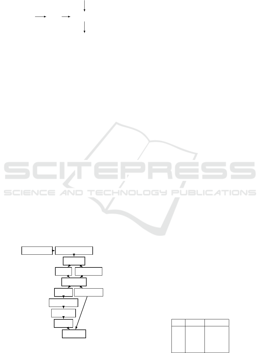
Batch (6000) Minibatch (100)
Sample i
Image
Quaternion
Rotate ψ
C
Image’
Quaternion’
Background
Grayscale
Image”
Sample’ i
Figure 8: Image processing during the minibatch creation:
the third angle ψ
C
is generated on the fly before the image
is flattened to obtain a gray level matrix.
the geodesic distance between the predicted and the
ground truth quaternion coming from (1).
G = |cos
−1
(2hq
P
,q
T
i
2
− 1)| (5)
The geodesic distance shows the smallest transforma-
tion needed to align the prediction with the truth and
can be seen as a cumulative Euler angle error for each
sample. Thus it is expected to be higher than any com-
ponents of E.
For the training phase we use a Nesterov momentum
backpropagation with an initial learning rate of 0.001
decreased through the epochs and a 0.9 momentum.
The λ regularization weight is set to 0.001 as well
as β. The implementation is Python-based with a
Theano+Lasagne framework. The training dataset is
build with a Blender rendering pipeline and learned
on a Nvidia Tesla P100 in roughly 10 hours. The
parameters giving the best score for the validation
dataset are kept for the test phase.
4.2 Results
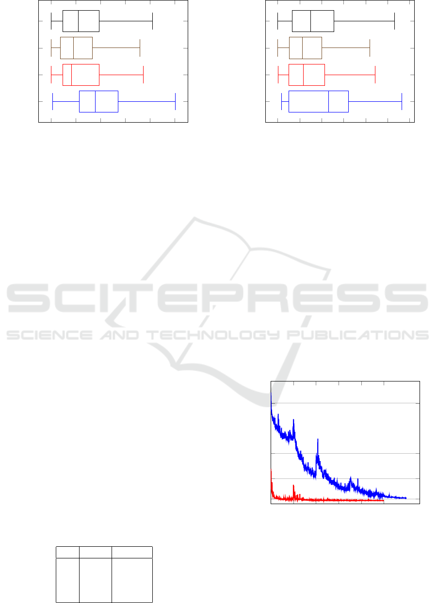
Looking at the results in Table 1 we are able to es-
timate both φ
C
and θ
C
with an average accuracy of
3
◦
when only the two first angles are learned with a
random background. The last estimated angle ψ
C
can
also be retrieved for an unitary quaternion since it can
represent any rotation composition. However we see
that the mean ψ
C
value is high because no variability
on it has been seen in the training dataset (Figure 9).
As expected, the geodesic error is the highest because
it represents an Euler angle cumulative error.
When the third angle ψ
C
is learned, we observe that
its distribution gets a larger prediction uncertainty
than in the two angles scenario but has a lower mean
(Figure 10). With a 6
◦
resolution for φ
C
and θ
C
and
10
◦
for ψ
C
, the angle error medians are under 3
◦
which shows that the network is performing the ex-
pected regression task and do not tend to classify to
the nearest learned angle (Table ??). It is interesting
to note that in a two angles learning scenario, the net-
work converges really fast at 100 epochs under a 5
◦
error whereas the three angles learning scenario needs
more than 1000 epochs (Figure 11). Some samples
are shown with the associated geodesic error in the
Figure 12. The trained network has two max-pooling
Table 1: Pose estimation angle error with a two angles train-
ing.
.
mean median
E
φ
4.39
◦
2.0
◦
E
θ
1.93
◦
1.46
◦
E
ψ
9.24
◦
1.52
◦
G 3.3
◦
2.8
◦
ICPRAM 2018 - 7th International Conference on Pattern Recognition Applications and Methods
414
0 2 4
6
8 10
G
E
ψ
E
θ
E
φ
Angle error (
◦
)
Figure 9: Box-plot of the angle estimation errors with two
angles generated (ψ
C
, θ
C
).
layers (Figure 6) which are known to be invariant to
small rotations. Despite their abilities to reduce the
training time and complexity, they tend to constrain
the prediction capacities of the algorithm.
When estimating the object pose from real images,
the task remains challenging for we do not dispose
any telecentric dataset. Only a small number of views
with limited perspective effects can be fed into the
network. With an only rendered-based training, we
are still able to estimate the pose of the object with a
visually convincing precision (Figure 13). Even if we
do not have any ground truth information, the pose of
the object inside the real image can be roughly esti-
mated by the mean of a 3D modeler as in Figure 5.
With this information, the average Euler’s angles er-
ror reaches 22
◦
.
5 CONCLUSION
In this paper we proposed a convolutional neural net-
work performing a 3D pose regression of a known ob-
ject in a scene. We showed that once the network has
learned from rendered data, it can infer from rendered
images the three Euler’s angles with a 5
◦
accuracy de-
spite the max-pooling layers dropping the third angle
estimation performance.
Inside a real industrial bin, the parts can lie on each
other so that severe occlusions are likely to happen.
Table 2: Pose estimation angle error with a three angles
training.
mean median
E
φ
6.46
◦
3.0
◦
E
θ
2.8
◦
2.26
◦
E
ψ
6.56
◦
2.31
◦
G 5.14
◦
4.61
◦
0 2 4
6
8 10 12
G
E
ψ
E
θ
E
φ
Angle error (
◦
)
Figure 10: Box-plot of the angle estimation errors with
three angles generated (φ
C
, θ
C
,ψ
C
).
However, our network does not learn how to han-
dle these configurations. Some works already tackle
this issue with a loss function term handling an occlu-
sion factor (Doumanoglou et al., 2016). In a future
work, occlusions are going to be taken into account
among an instance segmentation algorithm also based
on a convolutional neural network to get an end-to-
end learning process. When the network is fed with
real image containing small perspective effects, the
estimated pose is visually convincing however the ac-
curacy exceeds 22
◦
. There are several factors to be
taken into account to outperform this score: a non-
constant background luminosity, noise, perspective
effects and textured backgrounds. In a future work,
we aim at learning perspective effects by associating
any quaternion estimations to the object (x, y) position
in the image plane.
0 200 400
600
800 1,000
5
25
50
100
Epochs
G angle error (
◦
)
Figure 11: Geodesic error of test batch during the two (red)
and three (blue) angles training phase. For the three angles
training, the third angle steps are reduced at 200, 400, 700
and 900 epochs.
3D Orientation Estimation of Industrial Parts from 2D Images using Neural Networks
415
G = 2.62
◦
G = 4.11
◦
G = 2.75
◦
G = 5.92
◦
G = 2.29
◦
G = 2.85
◦
G = 2.85
◦
G = 2.16
◦
Figure 12: Estimating the object pose from rendered im-
ages. Left: the truth image. Right: the rendered estimated
pose. The geodesic error is printed below.
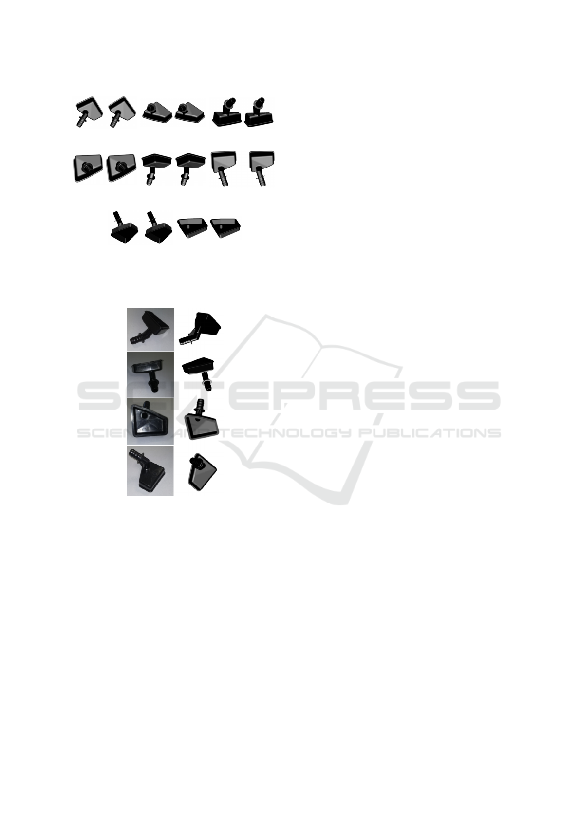
Figure 13: Estimating the object pose from real images.
Left: the real image. Right: the rendered estimated pose.
The estimation average accuracy reaches 22
◦
.
REFERENCES
Bay, H., Tuytelaars, T., and Gool, L. V. (2008). Surf :
Speeded up robust features. CVIU.
Bo, L., Ren, X., and Fox, D. (2012). Unsupervised feature
learning for rgb-d based object recognition. ISER.
Boucher, P. (2006). Points on a sphere.
Doumanoglou, A., Balntas, V., Kouskouridas, R., and Kim,
T.-K. (2016). Siamese regression networks with ef-
ficient mid-level feature extraction for 3d object pose
estimation. arXiv:1607.02257.
Gavrila, D. M. (1998). Multi-feature hierarchical template
matching using distance transforms. ICPR.
Gordon, I. and Lowe, D. G. (2004). What and where: 3d
object recognition with accurate pose. ISMAR.
Hinterstoisser, S., Holzer, S., Cagniart, C., Ilic, S., Kono-
lige, K., Navab, N., and Lepetit, V. (2011). Multi-
modal templates for real-time detection of texture-less
objects in heavily cluttered scenes. ICCV.
Hinterstoisser, S., Lepetit, V., Ilic, S., Fua, P., and Navab, N.
(2010). Dominant orientation templates for real-time
detection of texture-less objects. CVPR.
Hodan, T., Zabulis, X., Lourakis, M., Obdrzalek, S., and
Matas, J. (2015). Detection and fine 3d pose estima-
tion of texture-less objects in rgb-d images. IROS.
Honda, T., Igura, H., and Niwakawa, M. (1995). A handling
system for randomly placed casting parts using plane
fitting technique. IROS.
Huynh, D. (2009). Metrics for 3d rotations: comparison
and analysis. JMIV.
Kendall, A., Grimes, M., and Cipolla, R. (2015). Posenet:
A convolutional network for real-time 6-dof camera
relocalization. ICCV.
Lee, S., Wei, L., and Naguib, A. M. (2016). Adaptive
bayesian recognition and pose estimation of 3d indus-
trial objects with optimal feature selection. ISAM.
Lowe, D. G. (2004). Distinctive image features from scale-
invariant keypoints. IJCV.
Melekhov, I., Ylioinas, J., Kannala, J., and Rahtu, E. (2017).
Relative camera pose estimation using convolutional
neural networks. ACIVS.
Mitash, C., Bekris, K. E., and Boularias, A. (2017). A self-
supervised learning system for object detection using
physics simulation and multi-view pose estimation.
IROS.
Muja, M., Rusu, R. B., Bradski, G., and Lowe, D. G. (2011).
Rein-a fast, robust, scalable recognition infrastructure.
ICRA.
Schwarz, M., Schulz, H., and Behnke, S. (2015). Rgb-d
object recognition and pose estimation based on pre-
trained convolutional neural network features. ICRA.
Shotton, J., Glocker, B., Zach, C., Izadi, S., Criminisi, A.,
and Fitzgibbon, A. (2013). Scene coordinate regres-
sion forests for camera relocalization in rgb-d images.
CVPR.
Su, H., Qi, C. R., Li, Y., and Guibas, L. (2015). Render
for cnn: Viewpoint estimation in images using cnns
trained with rendered 3d model views. ICCV.
Tejani, A., Tang, D., Kouskouridas, R., and Kim, T.-K.
(2014). Latent-class hough forests for 3d object de-
tection and pose estimation. ECCV.
Wohlhart, P. and Lepetit, V. (2015). Learning descriptors
for object recognition and 3d pose estimation. CVPR.
ICPRAM 2018 - 7th International Conference on Pattern Recognition Applications and Methods
416
