
Verifiable Parameterised Behaviour Models
For Robotic and Embedded Systems
Vladimir Estivill-Castro and Ren
´
e Hexel
School of Information and Communication Technology, Griffith University, Nathan, QLD, Australia
Keywords:
Model-driven Engineering, Formal Methods, Robotic and Embedded Systems, Middleware.
Abstract:
Logic-labeled Finite-State Machines (LLFSMs) are Communicating Extended Finite State Machines that exe-
cute concurrently but with a predefined sequential schedule. This capacity has enabled effective formal verifi-
cation. Moreover, LLFSMs are very powerful tools for Model-Driven Software Engineering of the behaviour
of robotic and embedded systems. Although existing schedulers are capable of executing several instances of
the same model, the challenge is to provide mechanisms for creating parameterised models akin to function
calls. Since recent task planning algorithms can synthesise behaviours as LLFSMs with parameters and re-
cursion, it becomes necessary to have a useful operational tool that produces compiled executables for such
behaviours. Moreover, parameterisation allows replication of generic system components, reducing overall
design complexity. We produce safe mechanisms to set actual and formal parameters for multiple, concur-
rent instances of the same behaviour. We achieve the parameterisation of behaviour models analogous to a
procedural abstraction and discuss its advantages and disadvantages on formal verification.
1 INTRODUCTION
The prominent role of Model-driven software engi-
neering (MDSE) for robotics derives from industry
profiting from the promise of combining soft and
physical robots with emerging technologies and plat-
forms, e.g., for the Internet of Things (IoT), the Inter-
net of Services (IoS), and the Internet of Data (IoD);
and is propelled further by the promises of ubiquity
and scalability of Cloud Computing. The challenge,
thus, is to apply the power of abstract behaviour mod-
els in a systematic, reliable, and scalable form. More-
over, this kind of scalability has prompted modular
robots (Arney et al., 2010), that is, a robot that can
be composed of several physical parts. In such a sys-
tem, the number of copies or parts of the same kind
can be flexibly adjusted, not only prior to deployment,
but even during operation. Therefore, it is natural
to consider that the specified behaviour of modular
components should also be modular and would utilise
MDSE (Arney et al., 2010).
Logic-labeled finite-state machines (LLFSMs) are
a comprehensive mechanisms for modelling be-
haviour in robotics and embedded systems. LLF-
SMs can be considered to be inspired by the Timed
Finite-State Machines (t-fsms) that work as building
blocks of Brooks’ subsumption architecture (Brooks,
1986) as they can very well represent the LISP-
based textual language in which t-fsms were de-
scribed (Mataric, 1992; Brooks, 1990). A simi-
lar type of robotic behaviour description has been
presented for Teleo-reactive systems (Nilsson, 2001)
and Situated Automata (Rosenschein and Kaelbling,
1995). LLFSM concurrent execution offers deter-
ministic scheduling and allows the design of time-
triggered systems (Kopetz, 1993). Such determinism
has several advantages. In particular, the behaviour
of a system composed of LLFSMs is much more pre-
dictable, ensuring reliability. In fact, the predictive
schedule reduces the state explosion of uncontrolled
concurrency enabling formal verification and model
checking. It also enhances the confidence in any val-
idation performed. Therefore, LLFSMs can naturally
be incorporated into a test-driven-development frame-
work, making test failures significantly more repro-
ducible. Moreover, this sequential execution liber-
ates the designer of challenges related to concurrency,
such as race conditions, as at any given point in time,
only one LLFSM in the arrangement is executing,
making the execution of its ringlet atomic. The al-
ternative to LLFSMs are event-driven statecharts de-
rived from Harel’s State Charts (Harel and Naamad,
1996; Harel and Politi, 1998). This were incorporated
into OMT and later into UML. In these even-driven
364
Estivill-Castro, V. and Hexel, R.
Verifiable Parameterised Behaviour Models - For Robotic and Embedded Systems.
DOI: 10.5220/0006573903640371
In Proceedings of the 6th International Conference on Model-Driven Engineering and Software Development (MODELSWARD 2018), pages 364-371
ISBN: 978-989-758-283-7
Copyright © 2018 by SCITEPRESS – Science and Technology Publications, Lda. All rights reserved

finite-state models transitions are labeled by events.
We note that an event-driven system is typically based
on a software architecture built around stimuli-driven
call-backs or interrupts, a subscribe mechanism and
listeners that enact such call-backs. Reacting to
stimuli in this way implies uncontrolled concurrency
(e.g. using separate threads or event queues). Lam-
port (Lamport, 1984) provided fundamental proofs
of the limitations of event-driven systems. Reactive-
systems are responsive systems without much pro-
cessing, as opposed to deliberative systems (which
reason, plan, learn). Real-time systems are required to
meet time-deadlines in response to stimuli and time-
triggered systems have been shown very effective for
this (Kopetz, 1993). Therefore, although closely re-
lated, these terms are not the same, our preference for
LLFSMs is supported by the work of Lamport (Lam-
port, 1984) that provides solid reasons why real-time
systems may be better served by time-triggered sys-
tems and pre-determined schedules, rather than the
unbounded delays that may occur in event-driven sys-
tems.
The clfsm
1
scheduler executes an arrangement
of compiled LLFSMs, with the capacity to upload
and suspend LLFSM that represent behaviours dur-
ing runtime (Estivill-Castro and Hexel, 2016). The
clfsm scheduler offers very efficient, in-memory,
data-centric communication between different be-
haviour modules. This works very well if the num-
ber of listeners for a message are known well before
compile-time, but does not work so well if the role of
consumer and producers is to be decided at run-time.
Task planning technology has advanced signif-
icantly. Now, generic plans that solve generic
task planning problems can be synthesised as logic-
labeled finite-state machines with parameters and re-
cursion (Segovia-Aguas et al., 2016). This poses
the challenge of executing these behaviours as com-
piled routines on board a robot, even where several
instances are deployed recursively. Parameterisation
brings the challenge that the middleware cannot stati-
cally determine senders and receivers. Moreover, the
number of LLFSMs in an arrangement can dynam-
ically vary, e.g., through recursive invocation. The
missing link to improve communication, is that invo-
cation of a behaviour (modelled by a LLFSMs) should
be similar to a procedure or function call.
This paper provides such a model, demonstrated
first with the original that clfsm provides and then
proposing the semantics that parameterised LLFSM
invocations should have.
1
Available at http://mipal.net.au/downloads.php
2 INSTANTIATING SUSPENDED
MACHINES
An arrangement of parameterised LLFSMs can be de-
fined dynamically. LLFSMs can be loaded and un-
loaded by request from another machine. This mech-
anism is similar to the suspend/restart mechanism.
However, in the case of unload, the machine is re-
moved from the arrangement, while the load mecha-
nism adds the named LLFSM to the arrangement. We
introduce a variant we name load suspended. The se-
mantics of this new command is similar to the previ-
ous load command with the exception that rather than
loading a LLFSM that executes from the initial state,
with load suspended the child machine is set with its
suspended state as the current state.
Because a LLFSM can be loaded more than once,
LLFSM instances can be logically replicated in an ar-
rangement to execute concurrently, but, as we men-
tioned earlier, this facility was limited to communi-
cation patterns where the total number of LLFSM
was predictable at compilation time to create con-
trol/status communication messages.
We introduce the concept of setting parameters for
a loaded LLFSMs from a caller LLFSM. With this fa-
cility, we can now treat LLFSMs as a function call or
procedure invocation, precisely suitable to enact the
Hierarchical Finite State Controllers inferable with
task planning (Segovia-Aguas et al., 2016).
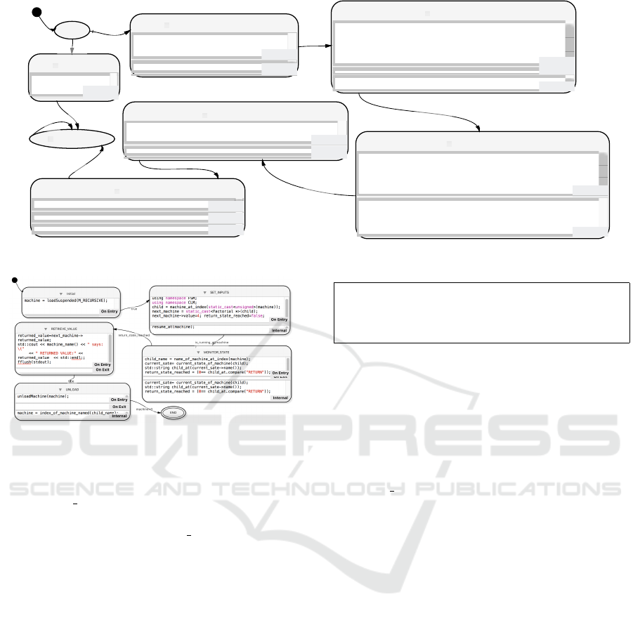
To demonstrate this facility and illustrate its se-
mantics, we present an example where we recursively
compute the factorial (Fig. 1). The Initial state of
this recursive LLFSM has two transitions. If the
value of its parameter (the variable value) is zero, the
returned value will be set to 1 (state END), and no
further recursion will occur (the machine will pause
in its RETURN state until its caller collects the return
value and such caller unloads the machine).
More interestingly, when the value of the in-
put parameter is greater than zero, the LLFSM
will use the loadSuspended command to load a
new instance of itself (in the OnEntry section
of the LOAD MYSELF SUSPENDED state). The
SET INPUTS state obtains a reference to the recently
loaded and, importantly, suspended machine and sets
the parameter to one less than the current value
(OnEntry section). The caller then requests that the
child resumes (Internal section) and once the child is
running (is running() predicate of the transition), it
will transition to the state MONITOR STATE.
The state MONITOR STATE retrieves the current
state of the child machine, exiting if the child is in
the RETURN state. Once that happens, the caller re-
trieves the returned value from the local variable of
Verifiable Parameterised Behaviour Models - For Robotic and Embedded Systems
365
Initial
returned_value =1;
On Entry
On Exit
Internal
END
RETURN
machine = loadSuspended(M_RECURSIVE);
On Entry
On Exit
Internal
LOAD_MYSELF_SUSPENDED
using namespace FSM;
using namespace CLM;
child = machine_at_index(static_cast<unsigned>(machine));
next_machine = static_cast<Factorial *>(child);
next_machine->value=value-1; return_state_reached=false;
On Entry
On Exit
resume_at(machine);
Internal
SET_INPUTS
child_name = name_of_machine_at_index(machine);
current_sate= current_state_of_machine(child);
std::string child_at(current_sate->name());
return_state_reached = (0== child_at.compare("RETURN"));
On Entry
On Exit
current_sate= current_state_of_machine(child);
std::string child_at(current_sate->name());
return_state_reached = (0== child_at.compare("RETURN"));
Internal
MONITOR_STATE
returned_value=value* next_machine-> returned_value;
On Entry
On Exit
Internal
RECORD_VALUE
unloadMachine(machine);
On Entry
On Exit
machine = index_of_machine_named(child_name);
Internal
UNLOAD
0==value
value>0
true
true
true
is_running_at(machine)
retur n_state_ reache d
true
machine<0
Figure 1: Recursive LLFSM for computing the factorial function f (n) = n!.
Figure 2: The LLFSMs that invokes the recursive LLFSM
from Fig. 1.
the child LLFSM (accessible trough the LLFSM ref-
erence next machine). In the case of the factorial
function, the value this instance returns is the prod-
uct of value with the returned value of the callee
LLFSM. The subsequent state is the state UNLOAD
where the child LLFSMs is removed from the ar-
rangement. Once this succeeds, this invocation itself
parks in its RETURN state.
The top-level LLFSM that makes the invoca-
tion is presented in Fig. 2 and its simpler but illus-
trates the particular steps of calling another LLFSM
as a procedure or recursive function using the new
loadSuspended. While the child is suspended, the
formal parameters are filled with values. This was not
possible previously, as the child machine would run
concurrently after load with uninitialised parameters.
Correctness of the recursive factorial function can
be established by induction (Wand, 1980). Estab-
lishing formally that the LLFSM model (Fig. 1) is a
correct executable model can be achieved with tech-
niques to verify recursive programs (Huang et al.,
2009). Our tool does not currently implement control-
flow graphs but produces the corresponding Kripke
structure for the LLFSM except the loadSuspended
LTLSPEC
G(pc=OnEntry(Initial) & M0value=0 -> X( pc=OnEntry(END) )
| X( X( pc=OnEntry(END) ) )
| X( X( X( pc=OnEntry(END) ) ) )
)
Figure 3: NuSMV coding of the property that, when
value=0, the next state after Initial is state END.
instruction. Nevertheless, for this example, formal
verification can proceed as we can establish LTL and
CTL properties for the LLFSM in Fig. 1.
Property 1 If the input value is zero, then all
paths lead to the RETURN state and the variable
returned value is 1 for all future states.
We can establish that, in this case (value=0), all
paths only use END once and followed by the state
RETURN, and they do not use any other state. For
a small illustration, Fig 3 shows the LTL formula
we used in NuSMV to verify that in no more than 3
Kripke states, the LLFSM of Fig. 1 reaches the state
END from the Initial state. Similarly, with our current
compiler that generates Kripke structures, we can use
NuSMV to establish that if the input value is greater
than zero, then the states executed are those on the
path and in the path’s sequence shown by the model.
However, the new loadSuspended offers a non-
blocking execution, much more general than the
vanilla invocation of a sub-routine with the semantics
for recursion of an invocation stack. In traditional,
imperative languages, the invocation of a subroutine
blocks the calling code at the point of invocation un-
til the subroutine terminates and returns. We demon-
strate the additional versatility of a non-blocking call
in the following examples.
MODELSWARD 2018 - 6th International Conference on Model-Driven Engineering and Software Development
366
Initial
VrepHexapodMotion a_motion = hexapod_motion->get();
VrepHexapodLegMotion legMotion =
VrepHexapodLegMotion(V_REP_HEXAPOD_RAISE);
a_motion.set_theLegMotions(legMotion , I_am );
hexapod_motion->post(a_motion);
On Entry
On Exit
Internal
RAISE_LEG
VrepHexapodMotion a_motion = hexapod_motion->get();
VrepHexapodLegMotion legMotion =
VrepHexapodLegMotion(V_REP_HEXAPOD_LEVEL);
a_motion.set_theLegMotions(legMotion , I_am );
hexapod_motion->post(a_motion);
On Entry
On Exit
Internal
LEVEL_LEG
VrepHexapodMotion a_motion = hexapod_motion->get();
VRepHexapodMotionCommand a_move =
(V_REP_HEXAPOD_WALK== spin_vs_walk) ?
reverse_move(I_am,direction) :
((V_REP_HEXAPOD_SPIN_BODY_COUNTER_CLOCKWISE== spin_vs_walk) ?
V_REP_HEXAPOD_CLOCKWISE : V_REP_HEXAPOD_COUNTER_CLOCKWISE );
VrepHexapodLegMotion legMotion = VrepHexapodLegMotion(a_move);
a_motion.set_theLegMotions(legMotion , I_am );
hexapod_motion->post(a_motion);
On Entry
On Exit
Internal
PUSH_OPPOSITE_DIRECTION
after_ms(FREQUENCY)&&0!=I_am%2
after_ms(FREQUENCY)&&0==I_am%2
after_ms(FREQUENCY)
after_ms(FREQUENCY)
after_ms(FREQUENCY)
after_ms(FREQUENCY)
VrepHexapodMotion a_motion = hexapod_motion->get();
VRepHexapodMotionCommand a_move =
(V_REP_HEXAPOD_WALK== spin_vs_walk)?
move(I_am,direction):
((V_REP_HEXAPOD_SPIN_BODY_COUNTER_CLOCKWISE== spin_vs_walk) ?
V_REP_HEXAPOD_COUNTER_CLOCKWISE :
V_REP_HEXAPOD_CLOCKWISE);
VrepHexapodLegMotion legMotion = VrepHexapodLegMotion(a_move);
a_motion.set_theLegMotions(legMotion , I_am );
hexapod_motion->post(a_motion);
On Entry
On Exit
Internal
SPIN_INTO_DIRECTION_OF_MOVEMENT
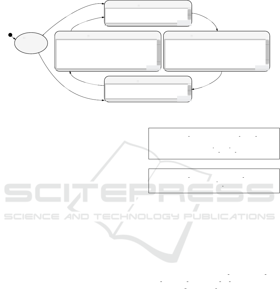
Figure 4: Executable model (as a parameterised LLFSM) for each leg of an n-legged robots. We can compose the walking
gait at any direction and also the spinning (clockwise or counter-clockwise) gait.
2.1 Hexapod Walk
We alluded earlier to the capacity to achieve scalabil-
ity using MDSE on modular robots. The gaits’ rhyth-
mic motion for an hexapod is a good example of the
generality of the behaviour model for legs. Although
our illustrations are for 6 legs, but they are applica-
ble to an arbitrary number of n legs placed around the
center of mass of the robot. In particular, when all
the legs are placed equidistant from the center of the
robot as if they were on a regular n-gon, it is easy to
imagine the gait that spins the robot clockwise. First,
the even numbered legs raise In the second stage, odd
legs use their body joint to push the robot clockwise
as they actually do a counter-clockwise turn of the
body joint. Simultaneously, the even legs are raised
and turn clockwise, advancing in the direction of the
spin. The third phase lowers the even legs while rais-
ing the odd legs and roles are reversed between these
groups of legs. In the fourth phase, it is now the legs
on the ground (the even legs) that push the body by
rotating counter-clockwise, while the raised ones (the
odd ones) rotate clockwise. An equivalent gait for
counter-clockwise rotation would simply reverse the
direction of joint rotations.
How does the robot walk in a particular orienta-
tion? Once more, the fundamental movement uses
the same four-stage leg movement. But, as opposed
to spinning, legs are now partitioned into two sides.
Those on the left will be performing motions to spin
clockwise, while those on the right of the center line
of motion will spin counter-clockwise. The robot will
walk because odd legs and even legs will have a phase
shift of two stages. So the robot will ‘row’ in the di-
rection of motion with even legs pushing back on the
ground, while the odd legs are raised and move for-
LTLSPEC
G(pc=OnEntry(LEVEL LEG) -> X( pc=OnEntry(PUSH OPPOSITE DIRECTION)
)
| X( X( pc=OnEntry(PUSH OPPOSITE DIRECTION) ) )
| X( X( X( pc=OnEntry(PUSH OPPOSITE DIRECTION) ) ) )
)
(a) NuSMV for state that follows.
LTLSPEC
G(pc=OnEntry(LEVEL LEG) -> X( pc!=OnEntry(RAISE LEG) )
| X( X( pc!=OnEntry(RAISE LEG) ) )
| X( X( X( pc!=OnEntry(RAISE LEG) ) ) )
)
(b) NuSMV for a section of a state that does not follow.
Figure 5: NuSMV coding of Property 2 and of Property 3 for
the executable LLFSM in Fig. 4.
ward, again, with the odd group of legs replaced by
the even in their role of pushing or advancing.
There are many more possible gaits. The point
we are illustrating is that linear and rotational leg
movements can be modelled as the fundamental
parameterised motion. Fig. 4 shows the fundamental
four states of a leg, RAISE LEG, LEVEL LEG,
SPIN AGAINST DIRECTION OF MOVEMENT, as
well as PUSH OPPOSITE DIRECTION. However,
deciding what is a push motion when the leg is down
or what is rotating back the leg when the leg is up
depends on three factors: (1) whether the hexapod is
walking or spinning, (2) whether this particular leg
is to the left or right of the direction of movement;
and (3) if we are spinning, then whether the motion
is a clockwise or counter-clockwise spin. Finally,
the phase of a leg motion depends on whether it
is an odd numbered leg or an even numbered leg.
Fig. 4 shows the parameterised executable LLFSM
for the motion of a leg. The motion starts raising
a leg or levelling a leg according to the group of
the leg (even or odd). From there on, all legs loop
through the same four states, and adjust the move
Verifiable Parameterised Behaviour Models - For Robotic and Embedded Systems
367

Figure 6: Section of the LLFSM that numbers the legs and sets the parameters based on the new action (and new direction)
the driver of the hexapod wants to take. All LLFSMs are then invoked concurrently (non-blocking).
when the leg is down or up according to the described
calculation. A video of a hexapod driven around
an area with spinning and walking can be seen at
https://youtu.be/60FgjRvZqsc. The parame-
terised LLFSM in Fig. 4 are launched as concurrent,
non-blocking calls with the corresponding parame-
ters. That is, the behaviour that conforms to the gait
in the case of the Hexapod invokes six instances of
Fig. 4 with the appropriate parameters.
2.2 Formal Verification of the
Executable Model
Formal verification of the behaviour for all legs in
Fig. 4 (which is an executable model) can be per-
formed with standard tools. Recall that the LLFSM
compiler derives the Kripke structure from the exe-
cutable model (Estivill-Castro and Hexel, 2013) as in-
put to NuSMV. We can readily verify that each state
is necessarily followed by the corresponding state
shown in Fig.4 and no other state before that. For ex-
ample, for the state LEVEL LEG, Fig. 5(a) shows the
LTL expression for the following property.
Property 2 It is globally true that, after the OnEntry
of state LEVEL LEG, in the next 3 Kripke states the
OnEntry of the state PUSH OPPOSITE DIRECTION
is executed.
Also, we need to show that no other part of any
other state is executed. A particular case is the fol-
lowing property.
Property 3 It is globally true that, after the
OnEntry of state LEVEL LEG happens, none of the
next 3 Kripke states are the OnEntry of the state
RAISE LEG.
Fig. 5(b) shows the NuSMV for Property 3. To com-
pletely verify the model, we would need a similar
property for every section of every other state besides
state PUSH OPPOSITE DIRECTION. And, of course,
for every state other than LEVEL LEG, the exercise
would require an analogue to Property 2, and all the
analogous LTL expressions to Property 3. However,
the point is that, with our tools, we can formally ver-
ify that, after initialisation, the states of the executable
LLFSM in Fig. 4 belong to the regular language
(LEVEL LEG PUSH OPPOSITE DITECTION RAISE LEG
SPIN AGAINST DIRECTION OF MOVEMENT)
+
.
2.3 Run-time Verification of the
Executable Model
As the purpose of this example was to show the flex-
ible non-blocking invocation of parameterised LLF-
SMs, we only show the most relevant states of the
controller LLFSMs that enable driving around of the
hexapod as illustrated in the video mentioned earlier.
Setting of parameters is shown in NUMBER LEGS
and RESTART LEG MACHINES, where the former
state assigns a number to each invoked LLFSM
(Fig. 6) and the latter actually performs the non-
blocking invocation.
However, since each LLFSM for the legs is
launched separately, there is a need to ensure syn-
chronisation. That is, the driver LLFSM needs to
check that all launched LLFSMs are running and then
synchronise them, before reading a new action (and
new direction) from the driver. For example, all even
legs (and similarly, all odd legs) must be in the same
state. This verification is rather different from the
verification performed with NuSMV earlier. In theory,
one could write the corresponding temporal logic for-
mula, but this would be particularly laborious. There-
fore, we illustrate the virtue by presenting an LLFSM
that verifies this aspect at run-time. The new mon-
itoring LLFSM will watch the state changes of the
six instances of LLFSMs for the hexapod. Recall that
all these are instances of the LLFSMof Fig 4, with
common parameters for the action (walking vs spin-
ning), but with a different leg number. The monitor-
ing LLFSM (different from the controlling LLFSM)
MODELSWARD 2018 - 6th International Conference on Model-Driven Engineering and Software Development
368
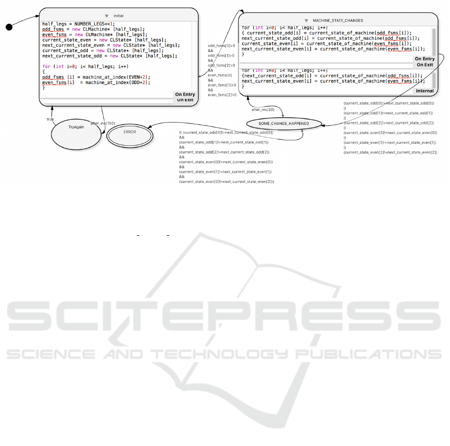
Figure 7: A monitoring LLFSM that inspects the states of the instances in Fig. 4 and checks the leg groups.
is shown in Fig. 7. The important aspect to notice is
that the transition from MACHINE STATE CHANGES
happens if any of the six LLFSMs has a state change
(the transition is whether the first, second, or third
odd-labelled leg LLFSM has a state change or the
first, second, or third even-labelled LLFSM has a state
change). In case not all machines involved had a state
change, the transition to the ERROR state fires. This
is also the virtue of LLFSMs’ deterministic sched-
ule, as all LLFSMs in the arrangement are guaran-
teed to receive the execution token before the moni-
toring LLFSM in Fig. 7 executes again. All LLFSMs
are executing concurrently, and despite non-blocking
calls that re-launched the leg controllers, synchroni-
sation is achieved without requiring explicit coordina-
tion (as required with open concurrency, e.g., through
semaphores, monitors, or other explicit synchronisa-
tion mechanisms that often render formal verification
impossible (Estivill-Castro and Hexel, 2013)). The
monitoring LLFSM in Fig. 7 is not necessary to con-
trol the hexapod. We use it for validation and in-
corporate it as part of a suitable software architec-
ture (Estivill-Castro and Hexel, 2016).
3 FUNCTIONAL
DECOMPOSITION
Functional decomposition is a major technique in
software design (Aggarwal and Simgh, 2008). Al-
gorithmic decomposition is a necessary part of
object-oriented analysis and design (Booch, 1994).
Functional decomposition is naturally used for
algorithmic-based system, where a problem is decom-
posed, broken into subproblems, whose solution is
then integrated into a final solution. This approach
to problem-solving and algorithm creation is exempli-
fied by divide and conquer (Cormen et al., 2009). Any
algorithm is fundamentally built from sequencing, se-
lection, and iteration of earlier defined algorithms (re-
call Structured Diagrams from Jackson’s Structured
Programming). The process of building abstractions
as subroutines is regularly practiced to build even
more sophisticated functions. We now illustrate that
our proposed parameterised behaviours act as build-
ing blocks of more sophisticated behaviour.
The example we chose is from the RoboCup Stan-
dard Platform League (http://spl.robocup.org), in par-
ticular, the entire soccer player behaviour, follow-
ing a top-down design. The behaviour must, at the
top level, maintain a few states, named Initial, Set,
Ready, Play, and Penalised. Suffice it to say that
the top behaviour therefore implements these states
as an LLFSM with corresponding transitions reacting
to the stimuli (e.g, UDP messages, a whistle, or even
buttons on the robot being pushed). Here, we focus
on the state of Ready, where a robot must reach a
legal position (usually its own half of the field) be-
fore game resumes (after a goal has been scored or
the first commencement of a period of play – see
https://youtu.be/6bzyf5fhTAQ). Thus, the state
of Ready is again broken down into sub-behaviours,
namely, to find a landmark (a goal), and identify-
ing whether that landmark is in the opponent’s or the
player’s half. Finding a goal (if not visible) corre-
sponds to scanning using the head, and if that is not
enough, to spin the whole robot around a bit (on the
spot). However, if the goal is visible, we need two
sub-behaviours, one to track the visible object with
the head, and one to align the body to the object.
Behaviour models are naturally designed using
Verifiable Parameterised Behaviour Models - For Robotic and Embedded Systems
369
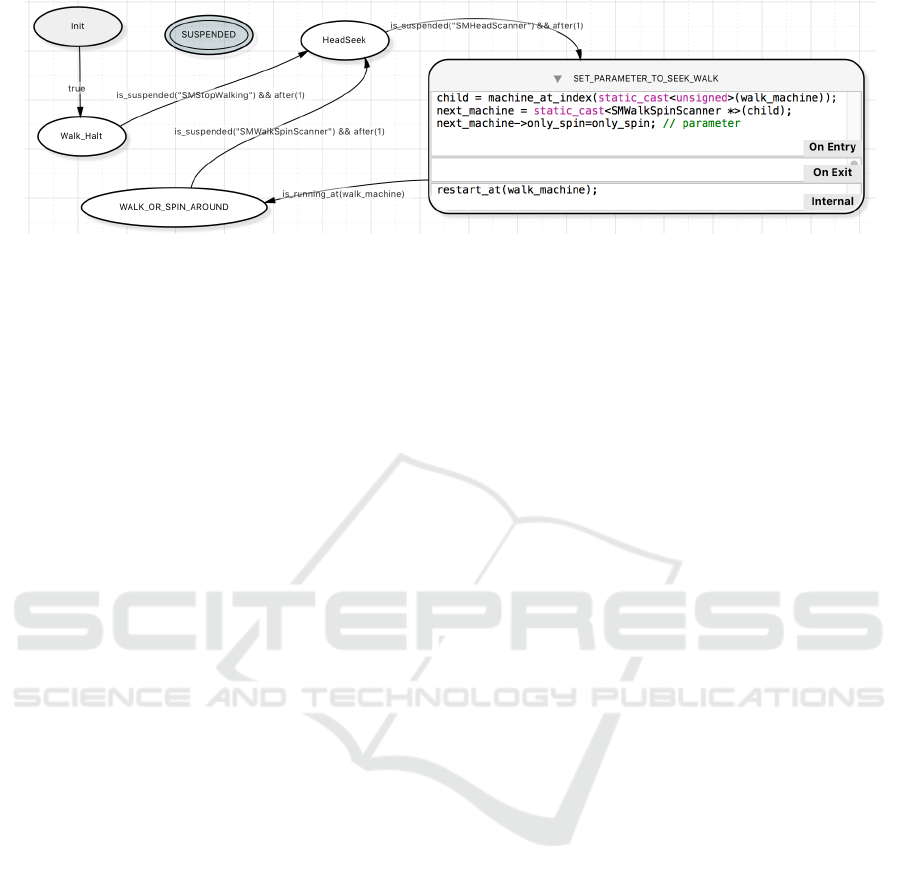
Figure 8: Behaviour searching for an object. A Boolean (formal) parameter controls whether to only spin on the spot or to
interleave a short walk. That parameter is passed along to a sub-behaviour to walk and/or spin.
functional decomposition. Figure 8 shows the land-
mark seeker LLFSM that was part of the behaviours
used by the MiPal team at RoboCup 2017 (Nagoya
Japan). Although functional decompositions are usu-
ally associated with Nassi-Shneiderman (NS) dia-
grams, or flowcharts or an activity diagram in UML,
LLFSM models are entirely suitable, particularly be-
cause they form executable models.
Importantly, Figure 8 demonstrates a parame-
terised model. The behaviour to search for a land-
mark uses 3 sub-machines, one to halt the walk, one
to scan using the head, and one to walk about, try-
ing to identify an object. The latter can be invoked
using a parameter. When finding landmarks for the
super-behaviour for Ready, it is only suitable to spin
on the spot (the designated starting position for the
robot). However, when finding the ball during Play,
it is important to alternate with walking backwards or
forwards to avoid missing the ball in a “dead spot”.
Thus, Figure 8’s behaviour invokes its sub-behaviour,
with a Boolean parameter to only spin or not.
This illustrates that parameterisation enables re-
factoring of behaviours, enabling their re-use for ini-
tially distinct sub-tasks in the hierarchy of decom-
position. That is the Seek behaviour becomes a re-
usable structure. Re-factoring improves the quality
of the implementation (Fowler, 1999), ensuring that
the generality of the code is extracted, and thus regu-
larly used in all cases, leading to fewer potential faults
(e.g., through cut-and-paste). Moreover, a generic be-
haviour needs to be formally verified only once.
The other aspect we illustrate with this example
is the flexibility of behaviour invocation as a non-
blocking call. Figure 9 shows the caller for Fig-
ure 8 that requests to focus on a goal. In fact, the
Seek behaviour generic, taking a parameter as to
what it is seeking for (a post, a ball, a goal, etc.).
This behaviour uses several sub-behaviours in addi-
tion to Seek. When the landmark is visible, two sub-
behaviours form what are essentially feedback-loop
controllers. The first is a behaviour tracks the object
with the neck of the robot, keeping the target object
centred as much as possible in the camera’s field of
view. The second sub-behaviour is a walk or spin,
that keeps the torso of the robot aligned with the ob-
ject (at the equilibrium point, the neck is centred look-
ing straight and the torso is also facing the target ob-
ject). The non-blocking nature of the invocation is ex-
ploited by the LLFSM in Figure 9 to abort the Seek
behaviour as soon as the landmark (or ball) becomes
visible. Similarly, if the landmark becomes invisible,
the sub-behaviours to track and follow the landmark
are aborted accordingly.
The SPL example illustrates the power of param-
eterised executable behaviours as LLFSMs. Sophis-
ticated, complex behaviours can be build bottom-up,
decoupled from an initial top-down design, thus al-
lowing re-factoring. While LLFSMs have a white-
board middleware as their default communication
mechanism, it is overkill to create communication
channels for every caller-callee pair, as that would re-
sult in many communication classes (or whiteboard
identifiers), specially if the same message is being
posted between several sender-receiver LLFSMs or
multiple instances of the same LLFSM. The white-
board is more suitable for a broadcast or knowledge
repository between individual components.
4 CONCLUSION
We showed the use of the loadSuspended capabil-
ity to create LLFSMs that can be invoked with pa-
rameters and enabling the construction of LLFSM-
sas recursive functions. As such, we believe we
have the only compiler for plans produced from new,
generic task planners. Moreover, we can generate
mechanisms for formal verification for all aspects of
the LLFSM semantics, including the loadSuspended
function. Also, our LLFSMs can themselves be used
to build monitoring LLFSMs for runtime verification.
This enables the generation of high level, executable
MODELSWARD 2018 - 6th International Conference on Model-Driven Engineering and Software Development
370
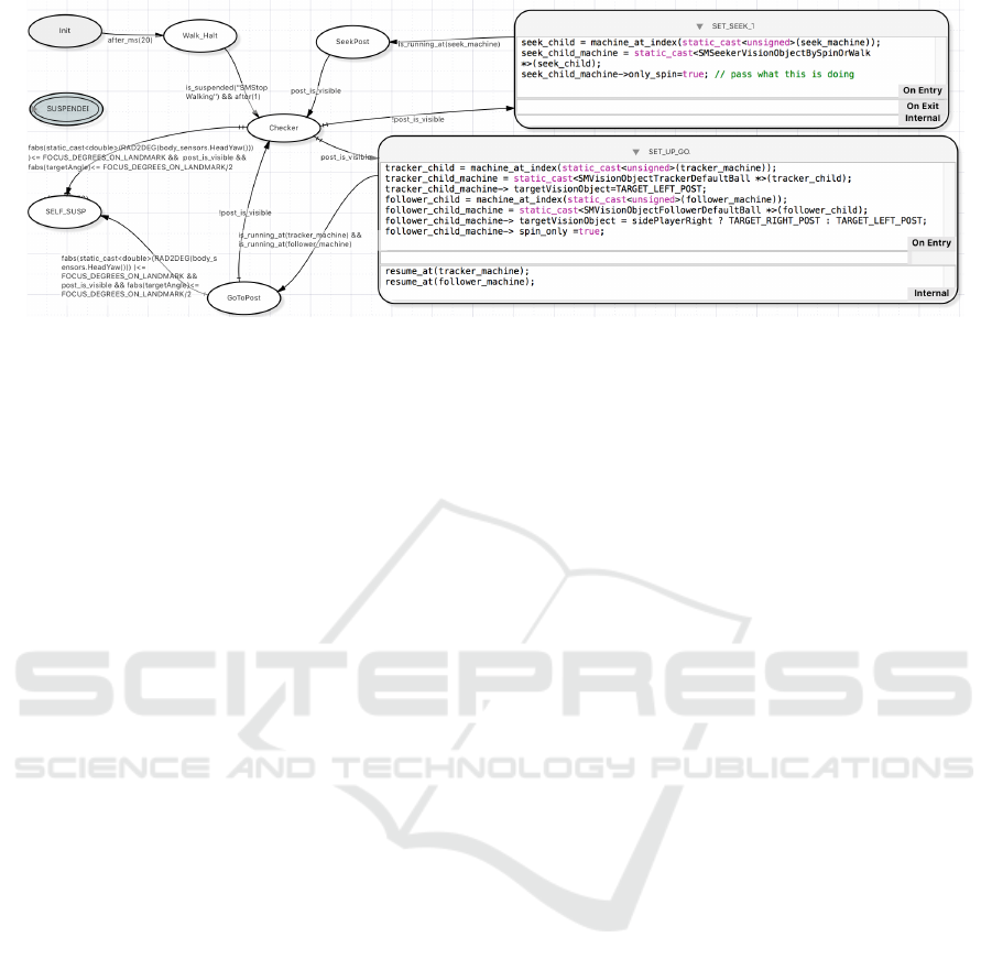
Figure 9: Behaviour as an LLFSM that follows and object, using Figure 8 when the object becomes invisible and two
sub-behaviours (invoked with suitable actual parameters) to track a visible object with the head and body.
behaviour models for robotic and embedded systems
that are modular and encapsulate design complexity.
REFERENCES
Aggarwal, K. K. and Simgh, Y. (2008). Software Engineer-
ing. New Age International, 3rd edition.
Arney, D., Fischmeister, S., Lee, I., Takashima, Y.,
and Yim, M. (2010). Model-based programming
of modular robots. 2010 13th IEEE Int. Symp.
Object/Component/Service-Oriented Real-Time Dis-
tributed Computing, p. 66–74.
Booch, G. (1994). Object-oriented Analysis and Design.
Benjamin/Cummings, Redwood Cita, CA, 2nd ed.
Brooks, R. (1986). A robust layered control system for
a mobile robot. IEEE J. Robotics and Automation,
2(1):14–23.
Brooks, R. (1990). The behavior language; user’s guide.
Tech. Rep. AIM-1227, MIT, AI Lab Pubs, Dep. of
Electronics and Computer Science.
Cormen, T. H., Leiserson, C. E., Rivest, R. L., and Stein, C.
(2009). Introduction to Algorithms. MIT Press.
Estivill-Castro, V. and Hexel, R. (2013). Arrangements
of finite-state machines semantics, simulation, and
model checking. Int. Conf. Model-Driven Engi-
neering and Software Development MODELSWARD,
p. 182–189, Barcelona, SciTePress.
Estivill-Castro, V. and Hexel, R. (2013). Module isola-
tion for efficient model checking and its application to
FMEA in model-driven engineering. ENASE 2013 -
8th Int. Conf. Evaluation of Novel Approaches to Soft-
ware Engineering, p. 218–225. SciTePress.
Estivill-Castro, V. and Hexel, R. (2016). Run-time veri-
fication of regularly expressed behavioral properties
in robotic systems with logic-labeled finite state ma-
chines. 2016 IEEE 5th Int. Conf. on Simulation, Mod-
eling, and Programming for Autonomous Robots -
SIMPAR, p. 281–288.
Fowler, M. (1999). Refactoring: Improving the Design of
Existing Code. Addison-Wesley, Boston, MA, USA.
Harel, D. and Naamad, A. (1996). The STATEMATE se-
mantics of statecharts. ACM T. Software Engineering
Methodology, 5(4):293–333.
Harel, D. and Politi, M. (1998). Modeling Reactive Sys-
tems with Statecharts: The STATEMATE Approach.
McGraw-Hill.
Huang, G.-D., Cai, L.-Z., and Wang, F. (2009). LTL model
checking for recursive programs. Automated Technol-
ogy for Verification and Analysis: 7th International
Symposium, ATVA, p. 382–396, Berlin. Springer.
Kopetz, H. (1993). Should responsive systems be event-
triggered or time-triggered? IEICE T. Information and
Systems, 76(11):1325.
Lamport, L. (1984). Using time instead of timeout for fault-
tolerant distributed systems. ACM Trans. Program.
Lang. Syst., 6(2):254–280.
Mataric, M. (1992). Integration of representation into goal-
driven behavior-based robots. IEEE T. Robotics and
Automation, 8(3):304 –312.
Nilsson, N. J. (2001). Teleo-reactive programs and the
triple-tower architecture. Electron. Trans. Artif. In-
tell., 5(B):99–110.
Rosenschein, S. J. and Kaelbling, L. P. (1995). A situated
view of representation and control. Artif. Intell., 73(1-
2):149–173.
Segovia-Aguas, J., Jim
´
enez, S., and Jonsson, A. (2016). Hi-
erarchical finite state controllers for generalized plan-
ning. 25th Int. Joint Conference on Artificial Intelli-
gence, IJCAI’16, p. 3235–3241. AAAI Press.
Wand, M. (1980). Induction, Recursion and Programming.
Elsevier Science, NY, USA.
Verifiable Parameterised Behaviour Models - For Robotic and Embedded Systems
371
