Segmentation of 3D Point Clouds using a New Spectral Clustering

Algorithm Without a-priori Knowledge

Hannes Kisner and Ulrike Thomas

Department of Robotics and Human-Machine Interaction, Chemnitz University of Technology, Germany

Keywords:

Spectral Clustering, Segmentation, Graph Laplacian, Point Clouds.

Abstract:

For many applications like pose estimation it is important to obtain good segmentation results as a pre-

processing step. Spectral clustering is an efﬁcient method to achieve high quality results without a priori

knowledge about the scene. Among other methods, it is either the k-means based spectral clustering approach

or the bi-spectral clustering approach, which are suitable for 3D point clouds. In this paper, a new method

is introduced and the results are compared to these well-known spectral clustering algorithms. When im-

plementing the spectral clustering methods key issues are: how to deﬁne similarity, how to build the graph

Laplacian and how to choose the number of clusters without any or less a-priori knowledge. The suggested

spectral clustering approach is described and evaluated with 3D point clouds. The advantage of this approach

is that no a-priori knowledge about the number of clusters is necessary and not even the number of clusters or

the number of objects need to be known. With this approach high quality segmentation results are achieved.

1 INTRODUCTION

In the last years many sensors were developed, which

are able to acquire 3D point clouds, e.g. Kinect

(Wasenm

uller and Stricker, 2016) or Stereo Systems

(Hirschm

uller, 2008). Since these sensors provide

point cloud data, scene analysis based on point clouds

became of high interest. Segmenting the scene into

various parts reduces the complexity and computati-

onal costs e.g. for object detection or pose estima-

tion. Due to the importance of acceptable segmen-

tation results, this paper investigates spectral cluste-

ring methods, also because they seem to represent a

good and robust alternative for scene segmentation.

A point cloud consists of an unsorted set of points

P = {p

,...,p

} with p

∈ R

which are either gained

by a single image or by acquisition of a sequence of

images, which then are registered to one point cloud.

In addition to point sets, curvature information can be

extracted by the principal component analysis (Rusu,

2009). Thus a set of estimated normal vectors is

available and is denoted as N = {n

,...,n

} throug-

hout this paper. Furthermore, colour information can

be used for each point HSV = {hsv

,...,hsv

}. For

many applications the quality of segmentation inﬂu-

ences the convergence speed for the used methods.

Spectral clustering approaches show acceptable re-

sults for segmentation processes. The bisection of

graphs based on similarities became very popular,

but requires a-priori information about the number of

clusters, or a suitable stopping-criterion. Instead, the

self-tuning algorithm is applied in order to reduce the

a priori knowledge (Zelnik-Manor and Perona, 2004).

This method outperforms other approaches regarding

the quality of segments. However, an efﬁcient imple-

mentation is important for the usability in applicati-

ons such as robotics. For this approach there are two

key challenges. Firstly, in order to build the Laplacian

graph, the similarity must be deﬁned. Secondly, an ef-

ﬁcient solution for estimating the number of clusters

must be found. Most spectral clustering algorithms

use a priori information about the number of clusters

and ignore the higher eigenvectors (see section 3.1),

but the usage of them can be exploited to obtain better

knowledge about the scene. The main advantage of

the new applied clustering method is that no a priori

knowledge about the scene is required, not even the

number of segments needs to be known in advance.

The results are compared to different spectral cluste-

ring methods. Section two presents related work and

section three describes the spectral clustering appro-

ach in detail. We describe different approaches and

compare them to our method, where higher ordered

eigenvectors are used to build a tree related to a de-

cision tree. The fourth section obtains the results and

the ﬁnal section concludes with an outlook.

Kisner, H. and Thomas, U.

Segmentation of 3D Point Clouds using a New Spectral Clustering Algorithm Without a-priori Knowledge.

DOI: 10.5220/0006549303150322

In Proceedings of the 13th International Joint Conference on Computer Vision, Imaging and Computer Graphics Theory and Applications (VISIGRAPP 2018) - Volume 4: VISAPP, pages

315-322

ISBN: 978-989-758-290-5

315

2 RELATED WORK

We deﬁne segmentation algorithms into region gro-

wing, kernel and graph cut based methods. Region

growing algorithms are one of the basic segmenta-

tion approaches (Preetha et al., 2012). Other seg-

mentation algorithms, that are similar to region gro-

wing algorithms, are watershed based methods for

3D mesh segmentation, where surface parameters like

curvatures and normals are used (Moumoun et al.,

2010). Another clustering algorithm ﬁts object pri-

mitives like planes and cylinders into the scene and is

available within the Point Cloud Library (PCL) (Rusu

and Cousins, 2011). For simple objects like cups,

boxes and convex parts this technique might work,

but often the basic shapes are unknown. Usually al-

gorithms that do not require a priori knowledge of

the scene are of high interest. Other techniques ex-

ist where only few parameters like the kernel band-

width and kernel proﬁle have to be adjusted in ad-

vance. A very widely used kernel based clustering

algorithm is the mean-shift algorithm (Comaniciu and

Meer, 2002). Spectral clustering is a method based on

spectral graph theory (von Luxburg, 2007). Another

similar approach is the normalized cut method (Shi

and Malik, 2000). This algorithm tries to ﬁnd a glo-

bal optimum by investigating the best possible cut on

the similarity graph. Spectral clustering is based on

the analysis of the eigenvectors of the graph Lapla-

cian (Fiedler, 1975). (Liu and Zhang, 2004) presented

results which achieve good segmentation of meshes.

Spectral clustering does not require strong assumpti-

ons on the input data, which is a great advantage, and

as another beneﬁt, it is superior in its performance,

at least in terms of the segmentation quality. Only

a few implementations of spectral clustering for 3D

point clouds are known, e.g. (Ma et al., 2010) and

(Funk et al., 2011). The ﬁrst implementation uses

the k-means algorithm to obtain the number of ex-

pected clusters, while the latter applies only recur-

sive bi-partitioning and uses the number of clusters

as stopping-criterion. One of the ﬁrst application of

spectral clustering applying surface normals is des-

cribed in (Cheng et al., 2011), but just like the other

methods, it needs the number of segments as input.

The work presented in this paper is based on spectral

clustering and extends the existing method to ﬁnd the

number of clusters automatically.

3 SPECTRAL CLUSTERING

Spectral clustering is based on the analysis of the

spectrum, i.e. the set of eigenvalues and eigenvec-

tors of the graph Laplacian. First of all, the point

cloud needs to be converted into a similarity graph

G = (V,E). Then the graph G is supposed to be

cut into two disjoint subgraphs (A,B ⊂ V ) such that

A ∪ B = V and A ∩ B =

0 by clustering. Each edge e

i j

is assigned a weight w

i j

describing the similarity be-

tween node i and node j. Then the costs of a cut are

described as the sum of the cutting edges

cut(A, B) =

∑

i∈A, j∈B

i j

. (1)

This implies that the best cut is given where the costs

of the cut (A,B) are minimized. Describing the graph

cut algorithm as minimization problem is not robust

regarding to outliers. Thus, a more sophisticated

cut criterion is the normalized cut suggested in (Shi

and Malik, 2000). The normalized cut takes both

the intra-cluster and the inter-cluster weights into ac-

count. Thus, isolated vertices are no longer able to

form independent groups. The next subsection shows

how the graph is constructed and introduces the met-

hods for calculating the weights.

3.1 Graph Construction and Weight

Calculation

The base for spectral clustering algorithm is the con-

struction of a graph that represents the whole point

cloud. First, for a reduction of the information, all

points were sorted into groups called supervoxels.

The PCL includes an implementation of the Voxel

Cloud Connectivity Segmentation Algorithm (VCCS)

(Papon et al., 2013). Points with the same geome-

tric and visual information were combined to small

regions. The relevant parameters are the colour (0.3),

spatial (0.7) and normal importance (1), in which the

values in the brackets represent their inﬂuence of each

feature. The described algorithm targets on a seg-

mentation by normals, whereby the value for normal

importance is much superior to the color importance.

Furthermore, the voxel and seed resolution depend on

the point cloud, but can be predeﬁned for each ca-

mera. In our case we set those parameters to values

resulting in around 500 supervoxels for a cloud with

300.000 points. An advantage of this algorithm is the

creation of a graph of the supervoxels. Every super-

voxel represents a vertex and if two supervoxels are

adjacent, an edge exists. Each supervoxel carries in-

formation about the average orientation and the cen-

troid. The following step is to calculate the weights of

the edges. Therefore we can make two assumptions.

The ﬁrst is to test whether two adjacent supervoxels i

and j are located on a plane, if so we assume that they

belong to the same object. Hence we declare them to

VISAPP 2018 - International Conference on Computer Vision Theory and Applications

316

be fully connected, which means the weight w

i j

= 1.

Therefore we assume two normals n

and n

to be ap-

proximately parallel if ∠(n

) ≤ 10

◦

. If this test

is true, we estimate a plane with the centroid c

and

. Afterwards we check if the distance between c

and the plane is less than three times the cloud reso-

lution, deﬁned by the mean value of each point and

its nearest neighbor. If so, we assume both super-

voxels as a plane. Another assumption is that convex

regions can be combined. This idea is used in (Lai

et al., 2009) and (Karpathy et al., 2013). They present

different criterions for convexity, that differ in some

special cases. Thus we combine these criterions to

get better results. This leads to consider two adjacent

supervoxel as convex cv(v

) = 1, if the following

equation helds

cv(v

) =











1 : (n

− n

)(d

i, j

) > 0 ∧

i, j

− (d

i, j

· n

)) ·n

> 0,

0 : otherwise,

(2)

where d

i, j

= c

− c

. Another possibility to calculate

the weight is to use the Gaussian function (von Lux-

burg, 2007):

Φ(r) = exp



−r

2σ



. (3)

Here, σ represents the Gaussian parameter and r re-

presents the Euclidean distance between the features

or properties of two vertices. To calculate r we use

the normal and color information. So for normals r

is calculated by r

= |n

− n

|. The color information

of the points arises from the camera sensor, they are in

the standard RGB format. It is difﬁcult to distinguish

between the brightness of each point, for that reason

we convert the RGB information to the HSV format.

Afterwards we get three color histograms (for each

color channel and) for each supervoxel. The next step

is to calculate the cross correlation between each of

the color channels for two combined vertices. After-

wards we build the average of all correlations corr

HSV

between two supervoxels. The next step is to convert

the range of corr

HSV

to the range of r

. Then we cal-

culate r

HSV

= |1 − 2 · corr

HSV

|. It leads to the weight

for each edge:

i j

(

1 ,if plane or convex

Φ(r

)+p

HSV

Φ(r

HSV

)

HSV

,otherwise

(4)

where p

and p

HSV

represent the weight for each fe-

ature (normally p

+ p

HSV

= 1). In our algorithm we

use a higher fraction for the normals (p

= 0.8). The

next subsection describes the normalized graph cut

method and its relation to spectral clustering.

3.2 Normalized Graph Cuts

According to the assigned weights of each edge, let

the degree of a vertex v

∈ V be d

∑

j=1

i j

with n =

|V | and let the volume of a subset A ⊂ V be deﬁned

as vol(A) =

∑

i=1

. The volume can be seen as the

density of a subset A. The normalized cut criterion

minimizes the similarity between the groups while it

maximizes the similarity within the groups. This two-

way normalized cut criterion can be expressed by

Norm cut(A, B) =

cut(A, B)

Vol(A)

cut(A, B)

Vol(B)

. (5)

There is no known algorithm to solve the minimiza-

tion problem for balanced criteria like the normalized

cut in polynomial time. In the following section it will

be shown that the minimization problem can be sol-

ved numerically by using eigensolvers and techniques

of the spectral graph theory.

3.3 Graph Laplacians

The unnormalized Laplacian matrix is deﬁned as L =

D − W where D is a diagonal n × n matrix which

contains the degree of each vertex on its diagonal

i,i

= d

and W is the adjacency matrix that contains

information about the weights between the vertices

W = (w

i, j

)

i, j=1,...,n

. Hence, the matrix L with the ele-

ments l

i, j

is expressed by

i, j











,if i = j and e

i j

∈ E,

−w

i j

,if i 6= j,

0 ,if i 6= j and e

i j

/∈ E,

(6)

where L is indexed by the vertices v

and v

. From

(von Luxburg, 2007) we know that L has many pro-

perties:

• L is symmetric and positive semi-deﬁnite which

follows from the matrices D and W. Thus, all ei-

genvalues satisfy λ ≥ 0.

• A trivial solution of the minimization of the qua-

dratic form is given by the constant one vector.

• L provides n eigenvalues 0 = λ

≤ λ

≤ ... ≤ λ

According to this property, the ﬁrst non-trivial solu-

tion is the second smallest eigenvalue λ

. The cor-

responding eigenvector is called the Fiedler vector

(Fiedler, 1975). Fiedler recognized the dependency

between eigenvalues and the connectivity graph:

• λ

> 0 if the graph is connected, i.e. the terms of

Lf do not vanish.

• The multiplicity of λ

, 0 = λ

< λ

i+1

is equal to the

number of connected components (Fiedler, 1975).

Segmentation of 3D Point Clouds using a New Spectral Clustering Algorithm Without a-priori Knowledge

317

The Fiedler vector provides the optimal bisection of a

graph, by separating those with smaller values from

those with larger values. Therefrom the recursive

clustering method can be drawn. The relation be-

tween normalized cuts and spectral analysis can be

found in the quadratic form of L by using the indica-

tor vector f = ( f

,..., f

)

∈ R

thereby the cut(A,B)

(von Luxburg, 2007) can be concluded as

Lf =

∑

i, j=1

i j

− f

)

. (7)

Hence, the solution of the real valued minimization

problem for the normalized cut can be obtained by

solving the generalized eigenvalue system Lf = λDf.

The generalized eigenvalue problem might also be

transformed into D

−1

Lf = λf and L

norm

f = λf. To

solve this eigenvalue problem, we can choose an ei-

gensolver for the real symmetrical eigenvalue pro-

blem.

3.4 Clustering

After the graph construction we attempt to subdivide

our graph into different groups. Therefore we try to

ﬁnd groups with high weights and cut edges with low

weights. This leads to spectral analysis. Following

two different approaches are most common – a recur-

sive and an iterative solution. The following chapters

describe both approaches in detail.

3.4.1 Recursive Partitioning

Following the ﬁrst approach, the connectivity graph

is consequently bisected recursively by applying the

Fiedler vector on each subgraph. In consequence of

the real numbered Laplacian matrix, splitting by the

sign on the Fiedler-Vector, as described in (Hagen

and Kahng, 1992), might take on a smooth progres-

sion and they do not differ that much from each other.

Another heuristic is to choose the median of the va-

lues as splitting point. Then the recursion stops as

the variance is below a threshold or the number of ex-

pected clusters has been reached. For example, the

algorithm by (Hagen and Kahng, 1992) uses the nor-

malized cut and compares the results with a predeﬁ-

ned threshold. The recursive spectral clustering has

two major disadvantages. One is that the eigensol-

ver needs to be executed according to the recursion

depth and the second disadvantage is, that for some

algorithms the number of clusters has to be predeﬁ-

ned. This means a-priori information about the scene

is required.

Instead of subdividing the graph G recursively by

the Fiedler vector to avoid unstable results and expen-

sive computation, it is possible to obtain all partitions

by solving the eigenvalue problem at once.

3.4.2 Structure of the Graph Laplacian

There are various algorithms for the iterative proce-

dure depending on the used graph Laplacian. Before

explaining the iterative clustering method, it is neces-

sary to know details about the block diagonal matri-

ces. In the case of Cluster C being connected, well

separated components with a distance going to inﬁ-

nity, the matrix L can be rearranged in a matter that

all vertices which belong to a speciﬁc connected com-

ponent reside within a block on the diagonal of L.

Entries of an eigenvector which do not belong to the

cluster (i.e. block) are padded with zeros. Each sub-

matrix L

on the diagonal holds exactly one eigen-

vector corresponding to the eigenvalue 0, because it

is connected. The spectrum of L is the union of the

spectrum of each block L

. A common approach is

to form a matrix U ∈ R

n×C

which columns are the

ﬁrst C eigenvectors corresponding to the smallest ei-

genvalues of L and treating each row of U as a point

∈ U

in a C-dimensional subspace. In the ideal case

of a block diagonal matrix L, the points y

are loca-

ted on different orthogonal axes in the C-dimensional

subspace, if they belong to different subgraphs. Or

they are coincide at a certain point along an axis, if

they belong to the same subgraph L

. Thus, each

dimension of the subspace represents the afﬁliation

of a certain point to one possible cluster (von Lux-

burg, 2007). From this observation a simple method

to ﬁnd the number of clusters is to count the occur-

rence of the eigenvalue 0, corresponding to the num-

ber of connected components. Since this works only

if the clusters are well separated, a common appro-

ach is to look for a salient gap in the magnitude of the

eigenvalues. If the distance of the magnitude of two

eigenvalues is high compared to the other eigenvalues

of the ﬁrst C eigenvectors, then this indicates that the

higher of both eigenvectors attempts to cut connected

components, where it is wrong because of a strong co-

herence. While it is easy to ﬁnd a unique (eigen)gap

that maximizes 4λ = |λ

− λ

C−1

| for separated clus-

ters, it is hard or even impossible if the clusters are

not clearly separated.

3.4.3 Self-Tuning Algorithm

With the Self-tuning method it is possible to ﬁnd

the clusters automatically (Zelnik-Manor and Perona,

2004). This approach aims to recover the block diago-

nal structure of U. The eigenvector matrix

U ∈ R

n×C

is treated as the perturbed matrix U =

U + H (Davis-

Kahan theorem), with H

n×C

(von Luxburg, 2007).

VISAPP 2018 - International Conference on Computer Vision Theory and Applications

318

The Davis-Kahan theorem states that the difference of

the perturbed (canonical) and not perturbed subspaces

is bounded, and the differences of the subspaces can

be expressed by the canonical angles. Thus, the eigen-

vector matrix U is treated as the (nearly) diagonal ma-

trix

U rotated by an orthogonal matrix R ∈ R

C×C

such

that U =

UR. So, it is guaranteed that there exists a

rotation

R which recovers (nearly)

U. The remaining

problem is the selection of the unknown number of

clusters respectively the choice of the ﬁrst C smallest

eigenvectors. It now appears that taking too few ei-

genvectors will not span a full basis for the subspace.

Consequently, taking more eigenvectors might deliver

a better grade of diagonally. Taking too many eigen-

vectors results in more than one entry per row (Zelnik-

Manor and Perona, 2004). This observation results

in an incremental approach which takes the ﬁrst two

eigenvectors and tries to align them with the canoni-

cal coordinate system. After this has been done, the

next eigenvector is added to the already rotated ma-

trix and the previous step is repeated. This procedure

continues until a predeﬁned number of C has been re-

ached. C, i.e. the number of clusters, which provides

the best grade of diagonally is then selected (Zelnik-

Manor and Perona, 2004). The negative aspect for

this approach is the following: the higher the maxi-

mum number of C the more iteration will be execu-

ted. This leads to a rise in computational costs. If the

number is too low it is possible to ﬁnd a false num-

ber of clusters, which could be a result of too many

objects or the existence of a lot of outliers.

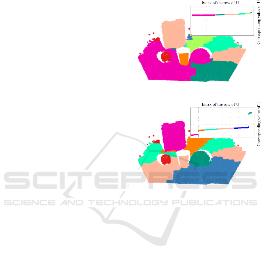
3.4.4 New Aproach

To overcome the issues mentioned above we combine

the concepts of both approaches. Firstly we use, as

mentioned by (Hagen and Kahng, 1992), one eigen-

vector to subdivide one graph into subgraphs. But as

mentioned in (Zelnik-Manor and Perona, 2004) we

also take a look at the higher eigenvectors. We know

that each row of U belongs to one voxel in the point

cloud. Like it is shown in Figure 1 There are diffe-

rent voxels in the point cloud labelled with different

colors that belong to the sorted rows of U. With a

look at Figure 2, we can see that for a higher eigen-

vector the corresponding points and rows have been

changed. This leads to the fact, that with different

eigenvectors we can build different subgraphs. As al-

ready described the higher the eigenvector the more

difﬁcult is the partitioning of the graphs. To overcome

this problem we are going to erase inessential points

of the graph. This leads to the following procedure,

as shown in Algorithm 1.

Firstly, we solve the unnormalised eigenvalue pro-

blem and use the Fiedler vector to divide the graph

Figure 1: Fiedler vector and the corresponding points of an

example point cloud.

Figure 2: 4th eigenvector and the corresponding points of

an example point cloud.

G into two subgraphs G

and G

with G

∩G

This is done by the calculation or the search of the

highest eigengap. Afterwards we take a look at the

third eigenvector. For the partitioning of G

we have

to delete the rows of U that belong to G

. Thus,

we consider only the necessary points. Then we get

further subgraphs. This calculation is done, until a

speciﬁc stopping-criterion is reached. Therefore we

can use an objective function like Equation 5 or, as

we did, a calculation of the average cut-size: Mean

cut(G

) = cut(G

)/n, where n represents

the number of cuts. If a set threshold τ is reached

the calculation or partitioning of the subgraph will be

stopped and we get the list of subgraphs. This corre-

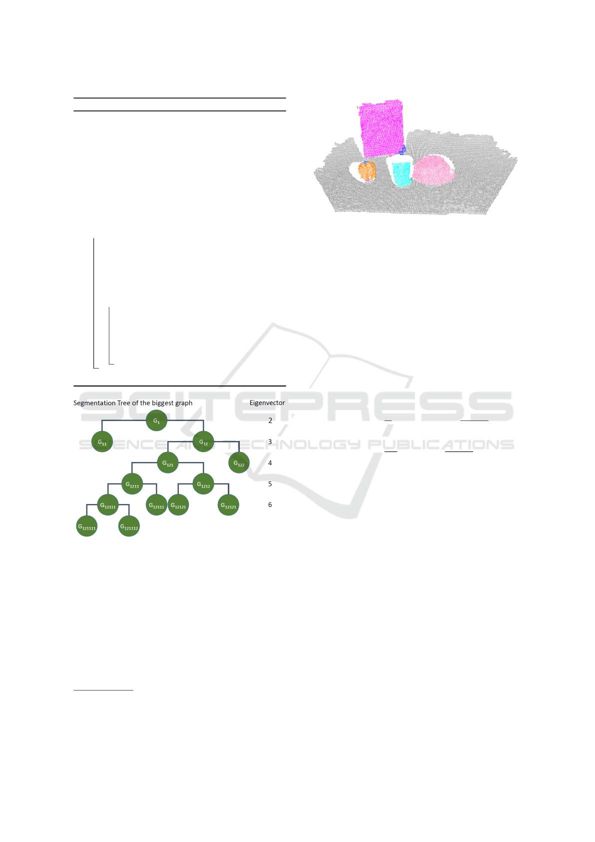
sponds to the clusters of the points as shown in Figure

4 and can be represented as a segmentation tree for

the scene as visualized in Figure 3. For this scene the

whole graph G

was separated into subgraphs using

up to six eigenvectors. The advantage of this method

is, that the eigenvalue problem needs to solved only

once, reducing the computation time.

Segmentation of 3D Point Clouds using a New Spectral Clustering Algorithm Without a-priori Knowledge

319

Algorithm 1: Clustering with higher eigenvectors.

Data: Graph G. Threshold τ

Result: List of subgraphs that reached the

threshold

1 Set up the degree matrix D ∈ R

n×n

with the

column sums of W ;

2 Calculate the Laplace matrix L and compute

eigenvalue problem for graph G;

3 Search Fiedler vector for 4λ

max

;

4 Calculate the objective function of the cut

with respect to 4λ

max

;

5 if objective function < τ then

6 Cut G into subgraphs;

7 Take the third eigenvector of G and

search the ﬁrst subgraph for 4λ

max

;

8 Calculate the objective function of the

new cut with respect to 4λ

max

;

9 if objective function < τ then

10 Cut subgraphs into further subgraphs;

11 Repeat seperatly for each subgraph

with the calculation of the objective

function of the next cut and the next

eigenvector;

12 end

Figure 3: The corresponding segmentation tree of an exam-

ple scene.

4 EVALUATION

For the evaluation the approach is tested with 3D

point clouds. Therefore we used the Modiﬁed Ob-

ject Segmentation Database (OSD-v0.2) proposed by

Alexandrov

. This dataset consists of different sce-

nes with box-like or cylindrical shaped objects. The

evaluation of such an algorithm is often difﬁcult and

https://github.com/PointCloudLibrary/data/tree/master/

segmentation/mOSD, originally proposed by (Richtsfeld

et al., 2012)

Figure 4: The resulting segmentation with the segmentation

tree from Figure 3 of an example scene.

depends on the needs for following algorithms. The-

refore we check different evaluation values. Firstly,

there is the calculation of correct labelled points. Fol-

lowing the above we check the ratio per ground truth

segment and count how many points are labelled cor-

rectly. Secondly, the number of different segments

per ground truth label are counted, which represents

the oversegmentation (OverSeg). In addition, we me-

asure the so called weighted overlap (WOv) and un-

weighted overlap (UWOv) for this evaluation; we im-

plemented the algorithms from (Arbelaez et al., 2011)

and (Hoiem et al., 2011). Here an overlap between the

ground truth data and each segment is calculated:

WOv(G, S) =

∑

∈G

| ·max

∈S



∩ S

∪ S



, (8)

UWOv(G, S) =

|G|

∑

∈G

max

∈S



∩ S

∪ S



, (9)

where a better segmentation results in values near to

one. Such criteria are used in recent work, e.g. by

(Stein et al., 2014) and evaluate the relative overseg-

mentation over the whole scene. Afterwards we build

histograms of the results and calculate the mean per

each evaluation criterion. The overall results for all

algorithms are listed in Table 1. Additionally we used

different values of τ for our algorithm to show its in-

ﬂuence. The results in table 1 and Figure 5 show

that in some situations the results of our segmenta-

tion have improved compared to the other algorithms,

which explains higher values respectively values near

to one in table 1. The explanation of the values for

oversegmentation is difﬁcult because the equation do

not consider outliers or the quantity of points per seg-

ment. A more detailed look shows that our algorithm

and the Self-tuning algorithm are challenged by con-

cave regions, like the inner part of a bowl or cup. This

is a result of the weight calculation, where we prio-

ritize convex regions. However, in this situation the

algorithm by Hagen demonstrates advantages which

could be a result of the threshold for the objective

VISAPP 2018 - International Conference on Computer Vision Theory and Applications

320

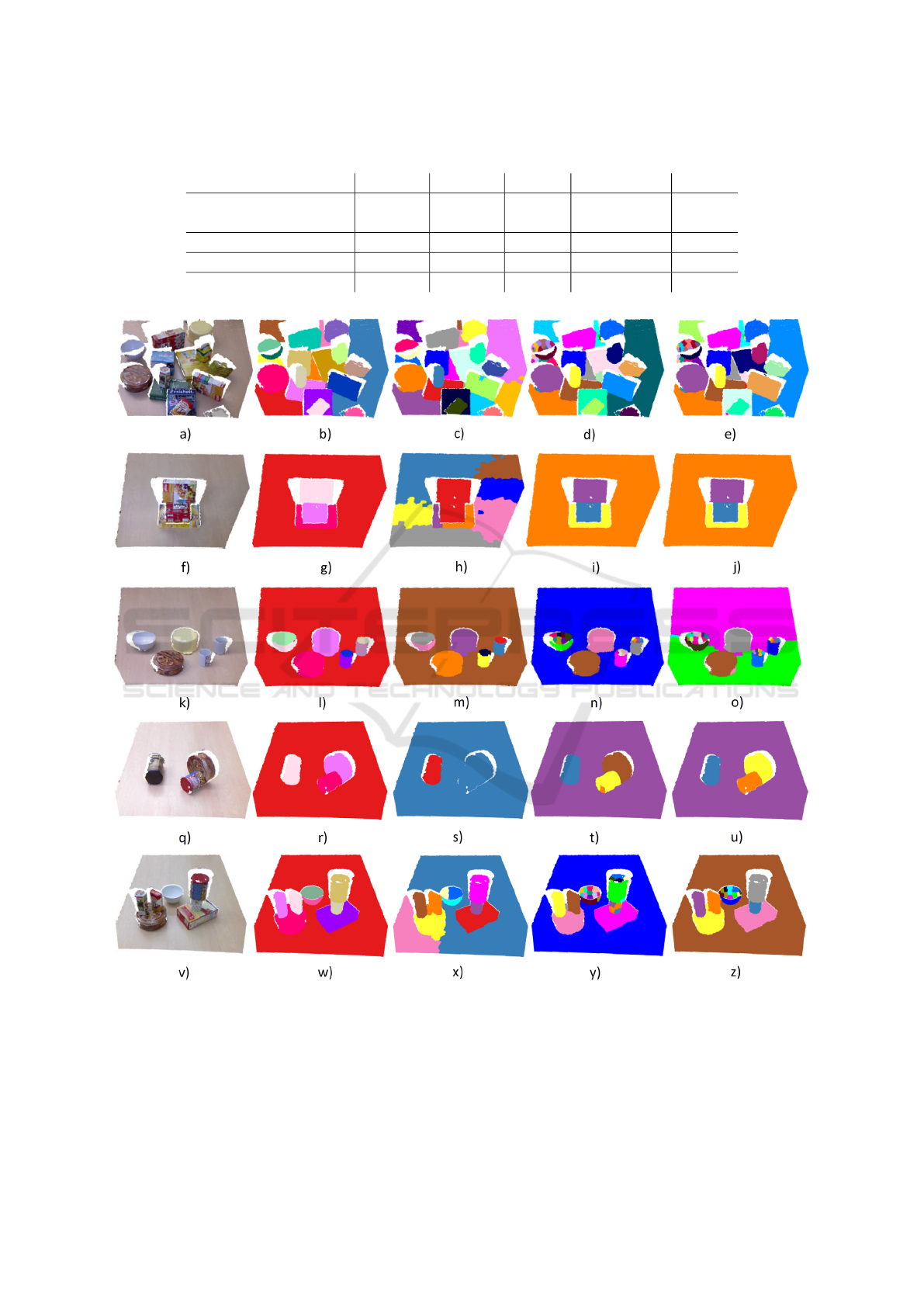
Table 1: Results for the whole dataset using different algorithms.

τ = 0.50 τ = 0.70 τ = 0.8 Self-Tuning Hagen

Fraction of correct

labeled points

0.9344 0.927 0.927 0.914 0.9342

Oversegmentation 2.66 2.8229 2.927 3.01 2.11

Weighted Covering 0.96 0.962 0.9613 0.9576 0.8653

Unweighted Covering 0.95 0.9522 0.9469 0.941 0.9336

Figure 5: Results of the segmentation algorithm. The ﬁrst column represents the original point cloud, the second the related

ground truth data, column three the results from the algorithm by Hagen and column four the results from the Self-Tuning

algorithm. The last column shows the results from our algorithm.

function. This threshold leads to more unstable re-

sults which means that sometimes there is a higher

over- or undersegmentation. Overall the algorithm,

that we developed, demonstrates more stable results

than the algorithm by Hagen and underlines advanta-

ges compared to the Self-Tuning algorithm.

Segmentation of 3D Point Clouds using a New Spectral Clustering Algorithm Without a-priori Knowledge

321

5 CONCLUSION

In this paper a new unsupervised learning approach

for 3D point cloud segmentation is suggested which

uses a spectral clustering with higher eigenvectors in

combination with a decision tree. We described how

the new spectral clustering approach can be imple-

mented to obtain high quality results. When applying

this solution no a priori knowledge about the scene,

not even the number of clusters, is necessary and it is

shown that only a threshold for an objective function

has to be adapted in a few cases. Thus, the spectral

clustering method outperforms many other clustering

algorithms. This approach is very robust with respect

to various input data. Moreover in comparison to ot-

her methods the eigenvalues and eigenvectors are only

calculated once and then inserted into the segmenta-

tion tree. In the future we will use this clustering met-

hod as a pre-processing step for object detection and

pose estimation. Further adaption can be considered

regarding the similarity weight.

ACKNOWLEDGEMENTS

This work is supported by the European Social Fund

(ESF) and the Free State of Saxony.

REFERENCES

Arbelaez, P., Maire, M., Fowlkes, C., and Malik, J. (2011).

Contour detection and hierarchical image segmenta-

tion. IEEE Transactions on Pattern Analysis and Ma-

chine Intelligence, pages 898–916.

Cheng, J., Qiao, M., Bian, W., and Tao, D. (2011). 3D

human posture segmentation by spectral clustering

with surface normal constraint. Signal Processing,

91(9):2204–2212.

Comaniciu, D. and Meer, P. (2002). Mean shift: a ro-

bust approach toward feature space analysis. IEEE

Transactions on Pattern Analysis and Machine Intel-

ligence, 24(5):603–619.

Fiedler, M. (1975). A property of eigenvectors of non-

negative symmetric matrices and its application to

graph theory. Czechoslovak Mathematical Journal,

25(4):619–633.

Funk, E., Grießbach, D., Baumbach, D., Ernst, I., Boer-

ner, A., and Zuev, S. (2011). Segmentation of large

point-clouds using recursive local pca. International

Conference on Indoor Positioning and Navigation.

Hagen, L. and Kahng, A. B. (1992). New spectral methods

for ratio cut partitioning and clustering. IEEE Tran-

sactions on Computer-Aided Design of Integrated Ci-

rcuits and Systems, 11(9):1074–1085.

Hirschm

uller, H. (2008). Stereo processing by semiglobal

matching and mutual information. IEEE Transacti-

ons on Pattern Analysis and Machine Intelligence,

30(2):328–341.

Hoiem, D., Efros, A. A., and Hebert, M. (2011). Recovering

occlusion boundaries from an image. International

Journal of Computer Vision, 91(3):328.

Karpathy, A., Miller, S., and Fei-Fei, L. (2013). Object

discovery in 3d scenes via shape analysis. In Interna-

tional Conference on Robotics and Automation.

Lai, Y.-K., Hu, S.-M., Martin, R. R., and Rosin, P. L. (2009).

Rapid and effective segmentation of 3D models using

random walks. Computer Aided Geometric Design,

26(6):665–679.

Liu, R. and Zhang, H. (2004). Segmentation of 3d mes-

hes through spectral clustering. In Proceedings of

the Computer Graphics and Applications, pages 298–

305. IEEE Computer Society.

Ma, T., Wu, Z., Feng, L., Luo, P., and Long, X. (2010).

Point cloud segmentation through spectral clustering.

In The 2nd International Conference on Information

Science and Engineering, pages 1–4.

Moumoun, L., Chahhou, M., Gadi, T., and Benslimane,

R. (2010). 3d hierarchical segmentation using the

markers for the watershed transformation. Internati-

onal Journal of Engineering Science and Technology,

2(7):3165–3171.

Papon, J., Abramov, A., Schoeler, M., and W

org

otter, F.

(2013). Voxel cloud connectivity segmentation - su-

pervoxels for point clouds. In Computer Vision and

Pattern Recognition (CVPR), 2013 IEEE Conference

on, pages 2027–2034.

Preetha, M. M. S. J., Suresh, L. P., and Bosco, M. J. (2012).

Image segmentation using seeded region growing. In

2012 International Conference on Computing, Elec-

tronics and Electrical Technologies, pages 576–583.

Richtsfeld, A., Morwald, T., Prankl, J., Zillich, M., and Vin-

cze, M. (2012). Segmentation of unknown objects in

indoor environments. In International Conference on

Intelligent Robots and Systems.

Rusu, R. B. (2009). Semantic 3D Object Maps for Everyday

Manipulation in Human Living Environments. PhD

thesis, Technische Universit

at M

unchen.

Rusu, R. B. and Cousins, S. (2011). 3D is here: Point Cloud

Library (PCL). In International Conference on Robo-

tics and Automation (ICRA), Shanghai, China.

Shi, J. and Malik, J. (2000). Normalized cuts and image

segmentation. IEEE Transactions on Pattern Analysis

and Machine Intelligence, 22(8):888–905.

Stein, S. C., Wrgtter, F., Schoeler, M., Papon, J., and Kul-

vicius, T. (2014). Convexity based object partitioning

for robot applications. IEEE International Conference

on Robotics and Automation, pages 3213–3220.

von Luxburg, U. (2007). A tutorial on spectral clustering.

Statistics and Computing, 17(4):395–416.

Wasenm

uller, O. and Stricker, D. (2016). Comparison of

kinect v1 and v2 depth images in terms of accuracy

and precision. In ACCV Workshops.

Zelnik-Manor, L. and Perona, P. (2004). Self-tuning

spectral clustering. In Advances in Neural Informa-

tion Processing Systems 17, pages 1601–1608. MIT

Press.

VISAPP 2018 - International Conference on Computer Vision Theory and Applications

322