Overcoming the Curse of Dimensionality

When Clustering Multivariate Volume Data

Vladimir Molchanov

and Lars Linsen

1,2

Jacobs University, Bremen, Germany

Westf

alische Wilhelms-Universit

at M

unster, M

unster, Germany

Keywords:

Multi-dimensional Data Visualization, Multi-ﬁeld Data, Clustering.

Abstract:

Visual analytics of multidimensional data suffer from the curse of dimensionality, i.e., that even large numbers

of data points will be scattered in a high-dimensional space. The curse of dimensionality prohibits the proper

use of clustering algorithms in the high-dimensional space. Projecting the space before clustering imposes a

loss of information and possible mixing of separated clusters. We present an approach where we overcome

the curse of dimensionality for a particular type of multidimensional data, namely for attribute spaces of

multivariate volume data. For multivariate volume data, it is possible to interpolate between the data points in

the high-dimensional attribute space based on their spatial relationship in the volumetric domain (or physical

space). We apply this idea to a histogram-based clustering algorithm. We create a uniform partition of the

attribute space in multidimensional bins and compute a histogram indicating the number of data samples

belonging to each bin. Only non-empty bins are stored for efﬁciency. Without interpolation, the analysis is

highly sensitive to the cell sizes yielding inaccurate clustering for improper choices: Large cells result in no

cluster separation, while clusters fall apart for small cells. Using tri-linear interpolation in physical space,

we can reﬁne the data by generating additional samples. The reﬁnement scheme can adapt to the data point

distribution in attribute space and the histogram’s bin size. As a consequence, we can generate a density

computation, where clusters stay connected even when using very small cell sizes. We exploit this result to

create a robust hierarchical cluster tree. It can be visually explored using coordinated views to physical space

visualizations and to parallel coordinates plots. We apply our technique to several datasets and compare the

results against results without interpolation.

1 INTRODUCTION

Visualization of multivariate volume data has become

a common, yet still challenging task in scientiﬁc vi-

sualization. Data sets come from traditional scien-

tiﬁc visualization applications such as numerical sim-

ulations, see VisContest 2008 (Whalen and Norman,

2008), or medical imaging, see VisContest 2010 (Vis,

2010). While looking into individual attributes can

be of high interest, the full phenomena are often only

captured when looking into all attributes simultane-

ously. Consequently, visualization methods shall al-

low for the investigation and analysis of the multidi-

mensional attribute space. The attribute space may

consist of measured and/or simulated attributes as

well as derived attributes including statistical proper-

ties (e.g., means, variances) or vector and tensor ﬁeld

properties (e.g., divergence, ﬁnite time Lyupanov ex-

ponent, diffusion tensor eigenvalues). Hence, we are

facing a multidimensional data analysis task, where

dimension here refers to the dimensionality of the at-

tribute space.

Multidimensional data analysis typically requires

some automatic components that need to be used

to produce a visual encoding. Typical components

are clustering approaches or projections from higher-

dimensional spaces into 2D or 3D visual spaces. Of-

ten, clustering and projections are combined to pro-

duce a visualization of a clustering result. The clus-

tering approach shall be applied ﬁrst to produce high-

dimensional clusters, which can be used as an input

for an improved projection. Unfortunately, clustering

in a high-dimensional space faces the problem that

points belonging to the same cluster can be rather

far apart in the high-dimensional space. This obser-

vation is due to the curse of dimensionality, a term

coined by Bellman (Bellman, 1957). It refers to the

fact that there is an exponential increase of volume

when adding additional dimensions.

The impact of the curse of dimensionality on prac-

Molchanov, V. and Linsen, L.

Overcoming the Curse of Dimensionality When Clustering Multivariate Volume Data.

DOI: 10.5220/0006541900290039

In Proceedings of the 13th International Joint Conference on Computer Vision, Imaging and Computer Graphics Theory and Applications (VISIGRAPP 2018) - Volume 3: IVAPP, pages 29-39

ISBN: 978-989-758-289-9

tical issues when clustering high-dimensional data is

as follows: Clustering approaches can be categorized

as being based on distances between data points or

being based on density estimates. However, only

distance-based clustering algorithms can effectively

detect clusters of arbitrary shape. Distance-based

clustering approaches require local density estimates,

which are typically based on space partitioning (e.g.,

over a regular or an adaptive grid) or on a kernel func-

tion. Both grid-based and kernel-based approaches

require the choice of an appropriate size of locality

for density estimation, namely, the grid cell size or

the kernel size, respectively. Using a too large size

leads to not properly resolving the clusters such that

clusters may not be separated. Hence, a small size is

required. However, due to the curse of dimensional-

ity, clusters fall apart when using a too small size and

one ends up with individual data points rather than

clusters thereof.

Attribute spaces of multivariate volume data are

a speciﬁc case of multidimensional data, as the un-

structured data points in attribute space do have a

structure when looking into the corresponding phys-

ical space. We propose to make use of this struc-

ture by applying interpolation between attribute-space

data points whose corresponding representations in

physical space exhibit a neighbor relationship.

The overall approach presented in this paper takes

as input a multivariate volume data set. First, it

applies an interpolation scheme to upsample the at-

tribute space, see Section 4 for the main idea, Sec-

tion 5 for an improved computation scheme, and Sec-

tion 6 for an amendment to handle sharp material

boundaries. The upsampled attribute space is, then,

clustered using a hierarchical density-based cluster-

ing approach, see Section 3. Based on the clustering

result, Section 7 describes how a combined visual ex-

ploration of physical and attribute space using coor-

dinated views can be employed. The results of the

approach are presented in Section 8 and its proper-

ties are discussed in Section 9. It is shown that our

approach manages to produce high-quality clustering

results without the necessity of tweaking the grid cell

size or similar. We also document that comparable re-

sults cannot be obtained when clustering without the

proposed interpolation step. The linked volume vi-

sualization, therefore, reﬂects the phenomena in the

multivariate volume data more reliably.

2 RELATED WORK

2.1 Multivariate Volume Data

Visualization

Traditionally, spatial data visualization focuses on

one attribute, which may be scalar, vector, or tensor-

valued. In the last decade, there was an increase on

attempts to generalize the visualization methods to

multivariate volume data that allow for the visual ex-

traction of multivariate features. Sauber et al. (Sauber

et al., 2006) suggested to use multigraphs to gener-

ate combinations of multiple scalar ﬁelds, where the

number of nodes in the graph increase exponentially

with the number of dimensions. Similarly, Woodring

and Chen (Woodring and Shen, 2006) allowed for

boolean set operations of scalar ﬁeld visualization. In

this context, Akiba and Ma (Akiba and Ma, 2007) and

Blaas et al. (Blaas et al., 2007) were the ﬁrst who

used sophisticated visualization methods and inter-

action in the multi-dimensional attribute space. Ak-

iba and Ma (Akiba and Ma, 2007) suggested a tri-

space visualization that couples parallel coordinates

in attribute space with volume rendering in physi-

cal space in addition to one-dimensional plots over

time. Blaas et al. (Blaas et al., 2007) use scatter

plots in attribute space, where the multi-dimensional

data is projected into arbitrary planes. Daniels II et

al. (Daniels II et al., 2010) presented an approach for

interactive vector ﬁeld exploration by brushing on a

scatterplot of derived scalar properties of the vector

ﬁeld, i.e., a derived multivariate attribute space. How-

ever, their interactive attribute space exploration ap-

proach does not scale to higher-dimensional attribute

spaces. Other approaches are based on statistics rather

than interactive visual feature extraction: J

anicke et

al. (J

anicke et al., 2007) use statistical measures to de-

tect regions of a certain behavior in multi-dimensional

volume data, while Oeltze et al. (Oeltze et al., 2007)

use correlation and principal component analysis to

visualize medical perfusion data.

Recently, there has been the approach to couple

attribute space clustering with visual interactive ex-

ploration of multivariate volume data. Maciejewski

et al. (Maciejewski et al., 2009) developed multi-

dimensional transfer functions for direct volume ren-

dering using 2D and 3D histograms and density-based

clustering within these histograms. Since interactions

with the histograms are necessary for visual anal-

ysis of the data, their approach is restricted to at-

tribute spaces of, at most, three dimensions. Linsen et

al. (Linsen et al., 2008; Linsen et al., 2009) proposed

an approach that can operate on multivariate volume

data with higher-dimensional attribute spaces. The at-

IVAPP 2018 - International Conference on Information Visualization Theory and Applications

tribute space is clustered using a hierarchical density-

based approach and linked to physical-space visual-

ization based on surface extraction. Recently, the ap-

proach was extended by Dobrev et al. (Dobrev et al.,

2011) to an interactive analysis tool incorporating di-

rect volume rendering. Dobrev et al. show that the

generated clustering result is often not as desired and

propose interactive means to ﬁx the clustering result.

In this paper, we make use of the same clustering ap-

proach, see Section 3, and show how we can improve

the results with the methods proposed here.

2.2 Clustering

Cluster analysis divides data into meaningful or use-

ful groups (clusters). Clustering algorithms can be

categorized with respect to their properties of being

based on partitioning, hierarchical, based on density,

or based on grids (Jain and Dubes, 1988; Han and

Kamber, 2006). In partitioning methods, data sets are

divided into k clusters and each object must belong to

exactly one cluster. In hierarchical methods, data sets

are represented using similarity trees and clusters are

extracted from this hierarchical tree. In density-based

methods, clusters are a dense region of points sepa-

rated by low-density regions. In grid-based methods,

the data space is divided into a ﬁnite number of cells

that form a grid structure and all of the clustering op-

erations are performed on the cells.

Hartigan (Hartigan, 1975; Hartigan, 1985) ﬁrst

proposed to identify clusters as high density clusters

in data space. Wong and Lane (Wong and Lane, 1983)

deﬁne neighbors for each data point in data space

and use the kth nearest neighbors to estimate density.

After deﬁning dissimilarity between neighboring pat-

terns, a hierarchical cluster tree is generated by ap-

plying a single-linkage algorithm. In their paper, they

show that the high density clusters are strongly con-

sistent. However, they do not examine modes of the

density function.

Ester et al. (Ester et al., 1996) introduced the DB-

SCAN algorithm. The ﬁrst step of the DBSCAN

algorithm is to estimate the density using an E ps-

neighborhood (like a spherical density estimate). Sec-

ond, DBSCAN selects a threshold level set MinPts

and eliminates all points with density values less than

MinPts. Third, a graph is constructed based on the

two parameters E ps and MinPts. Finally, high den-

sity clusters are generated by connected components

of the graph. The drawback is the need to deﬁne

appropriate parameters. Hinneburg and Keim in-

troduced the DENCLUE approach (Hinneburg and

Keim, 1998), where high density clusters are identi-

ﬁed by determining density attraction. Hinneburg et

al. further introduced the HD-Eye system (Hinneburg

et al., 1999) that uses visualization to ﬁnd the best

contracting projection into a one- or two-dimensional

space. The data are divided based on a sequence of

the best projections determined by the high density

clusters. The advantage of this method is that it does

not divide regions of high density.

Ankerst et al. (Ankerst et al., 1999) introduced the

OPTICS algorithm, which computes a complex hi-

erarchical cluster structure and arranges it in a lin-

ear order that is visualized in the reachability plot.

Stuetzle (Stuetzle, 2003) also used a nearest neighbor

density estimate. A high density cluster is generated

by cutting off all minimum spanning tree edges with

length greater than a speciﬁc parameter (depending

on the level-set value of the density function). Stuet-

zle and Nugent (Stuetzle and Nugent, 2007) proposed

to construct a graph whose vertices are patterns and

whose edges are weighted by the minimum value of

the density estimates along the line segment connect-

ing the two vertices. The disadvantage of this hierar-

chical density-based approach is that the hierarchical

cluster tree depends on a threshold parameter (level-

set value) that is difﬁcult to determine.

We use a hierarchical density-based approach that

computes densities over a grid. The main advantage

of our approach is the direct identiﬁcation of clusters

without any threshold parameter of density level sets.

Moreover, it is quite efﬁcient and scales well. The

main idea of the approach is described in Section 3.

For a detailed analysis and comparison to other clus-

tering approaches, which is beyond the scope of this

paper, we refer to the literature (Long, 2009).

2.3 Interpolation in Attribute Space

Our main idea is based on interpolation in attribute

space, which is possible due to a meaningful neigh-

borhood structure in physical space that can be im-

posed onto the attribute space. Similar observations

have been used in the concept of continuous scatter-

plots (Bachthaler and Weiskopf, 2008; Bachthaler and

Weiskopf, 2009; Heinrich et al., 2011; Lehmann and

Theisel, 2010; Lehmann and Theisel, 2011). Con-

tinuous scatterplots generalize the concept of scatter-

plots to the visualization of spatially continuous in-

put data by a continuous and dense plot. The high-

dimensional histograms we create can be regarded

as a generalization of the 2D continuous histograms

created by Bachthaler and Weiskopf (Bachthaler

and Weiskopf, 2008). It is a more difﬁcult prob-

lem to compute continuous histograms in higher-

dimensional spaces. However, in the end, we only

need a discrete sampling of the continuous histogram.

Overcoming the Curse of Dimensionality When Clustering Multivariate Volume Data

Hence, our computations do not aim at computing

continuous histograms, but rather stick to operating

on a discrete setting.

3 CLUSTERING

We present a hierarchical density cluster construction

based on nonparametric density estimation using mul-

tivariate histograms. Clusters can be identiﬁed with-

out any threshold parameter of density level sets. Let

the domain of the attribute space be given in form

of a d-dimensional hypercube, i.e., a d-dimensional

bounding box. To derive the density function, we spa-

tially subdivide the domain of the data set into cells

(or bins) of equal shape and size. Thus, the spa-

tial subdivision is given in form of a d-dimensional

regular structured grid with equidistant d-dimensional

grid points, i.e., a d-dimensional histogram. For each

bin of the histogram, we count the number of sample

points lying inside. The multivariate density function

is estimated by the formula

f (x) =

bin

n ·A

bin

for any x within the cell, where n is the overall number

of data points, n

bin

is the number of data points inside

the bin, and A

bin

is the area of the d-dimensional bin.

As the area A

bin

is equal for all bins, the density of

each bin is proportional to the number n

bin

of data

points lying inside the bin. Hence, it sufﬁces to just

operate with those numbers n

bin

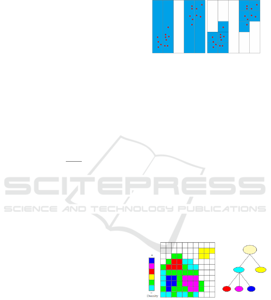
To estimate all non-empty bins, we use a parti-

tioning algorithm that iterates through all dimensions.

Figure 1 illustrates the partition process for a two-

dimensional data set: The ﬁrst dimension is divided

into 5 equally-sized intervals on the left-hand side of

Figure 1. Only four non-empty intervals are obtained.

These intervals are subsequently divided in the sec-

ond dimension, as shown on the right-hand side of

Figure 1. The time complexity for partitioning the

data space is O(nd), i.e., it can handle both data sets

with large number of samples n and data sets with

high dimensionality d.

Given the d-dimensional histogram, clusters are

deﬁned as largest sets of neighboring non-empty bins,

where neighboring refers to sharing a common vertex.

To detect higher-density clusters within each cluster,

we remove all cells containing the minimum number

of points in this cluster and detect among the remain-

ing cells, again, largest sets of neighboring cells. This

step may lead to splitting of a cluster into multiple

higher-density clusters. This process is iterated until

no more clusters split. Recording the splitting infor-

mation, we obtain a cluster hierarchy. Those clusters

Figure 1: Grid partition of two-dimensional data set: The

space is divided into equally-sized bins in the ﬁrst dimen-

sion (left) and the non-empty bins are further subdivided in

the second dimensions (right).

that do not split anymore represent local maxima and

are referred to as mode clusters. Figure 2 (left) shows

a set of non-empty cells with six different density lev-

els in a two-dimensional space. First, we ﬁnd the two

low-density clusters as connected components of non-

empty cells. They are represented in the cluster tree

as immediate children nodes of the root node (cyan

and yellow), see Figure 2 (right). From the cluster

colored cyan, we remove all minimum density level

cells (cyan). The cluster remains connected. Then,

we again remove the cells with minimum density level

(green). The cluster splits into three higher-density

clusters (red, magenta, and blue). They appear as chil-

dren nodes of the cyan node in the cluster tree. As

densities are given in form of counts of data points,

they are always natural numbers. Consequently, we

cannot miss any split of a density cluster when iterat-

ing over the natural numbers (from zero to the maxi-

mum density). The time complexity to create a hier-

archical density cluster tree is O(m

), where m is the

number of non-empty cells.

Figure 2: Left: Grid partition of two-dimensional data set

with six different density levels. Right: Respective density

cluster tree with four modes shown as leaves of the tree.

Figure 3 shows that the clustering approach is ca-

pable of handling clusters of any shape and that it

is robust against changing cluster density and noise.

Noise has been handled by removing all cells with a

number of sample points smaller than a noise thresh-

old. The data set is a synthetic one (Karypis et al.,

1999). Figure 4 shows the visualization of a cluster

IVAPP 2018 - International Conference on Information Visualization Theory and Applications

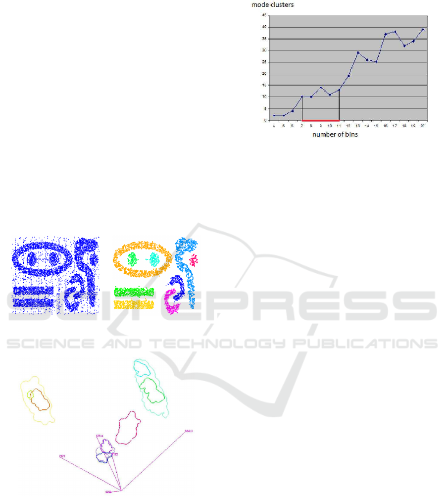
hierarchy for the “out5d” data set with 16,384 data

points and ﬁve attributes, namely, spot (SPO), mag-

netics (MAG), potassium (POS), thorium (THO), and

uranium (URA), using a projection in optimized 2D

star coordinates (Long, 2009). The result seems fea-

sible and all clusters were found without deﬁning any

density thresholds, but the choice of the bin size had

to be determined empirically in an interactive visual

analysis using coordinated views as described in this

paper. Figure 5 shows how sensitive the result is to the

bin size: Using smaller bin sizes merges some clus-

ters, while using larger sizes makes clusters fall apart.

The result in Figure 4 was obtained using the heuris-

tic that cluster numbers only vary slowly close to the

optimal bin size value (area marked red in Figure 4).

However, in practice one would not generate results

for the entire range of possible bin sizes for being able

to apply this heuristic. Instead, one would rather use

a trial-and-error approach, not knowing how reliable

the result is.

Figure 3: Clustering of arbitrarily shaped clusters. Left:

Original data set. Right: Histogram-based clustering result.

Figure 4: Visualization of cluster hierarchy in optimized 2D

star coordinates.

4 INTERPOLATION

Let the attribute values of the multivariate volume

data be given at points p

, i = 1,...,n, in physical

space. Moreover, let a

), j = 1,...,d, be the at-

tribute values at p

. Then, the points p

exhibit some

Figure 5: Sensitivity of clustering results with respect to the

bin size. The graph plots the number of mode clusters over

the number of bins per dimension.

neighborhood relationship in physical space. Typi-

cally, this neighborhood information is given in form

of grid connectivity, but even if no connectivity is

given, meaningful neighborhood information can be

derived in physical space by looking at distances (e.g.,

nearest neighbors or natural neighbors). Based on

this neighborhood information, we can perform an

interpolation to reconstruct a continuous multivari-

ate ﬁeld over the volumetric domain. In the follow-

ing, we assume that the points p

are given in struc-

tured form over a regular (i.e., rectangular) hexahe-

dral grid. Thus, the reconstruction of a continuous

multivariate ﬁeld can be obtained by simple trilinear

interpolation within each cuboid cell of the underly-

ing grid. More precisely: Let q be a point inside a

grid cell with corner points p

uvw

, u,v,w ∈ {0,1}, and

let (q

) ∈ [0,1]

be the local Cartesian coordi-

nates of q within the cell. Then, we can compute the

attribute values at q by

(q) =

∑

u=0

∑

v=0

∑

w=0

(1 −q

)

1−u

(1 −q

)

1−v

(1 −q

)

1−w

uvw

)

for all attributes ( j = 1,...,d). In attribute

space, we obtain the point (a

(q),...,a

(q)), which

lies within the convex hull of the set of points

uvw

),...,a

uvw

)), u,v,w ∈ {0,1}.

Now, we want to use the interpolation scheme to

overcome the curse of dimensionality when creating

the d-dimensional density histogram. Using the tri-

linear interpolation scheme, we reconstruct the mul-

tivariate ﬁeld within each single cell, which corre-

sponds to a reconstructed area in attribute space. The

portion r ∈ [0, 1] by which the reconstructed area in

attribute space falls into a bin of the d-dimensional

density histogram deﬁnes the amount of density that

should be added to the respective bin of the histogram.

Overcoming the Curse of Dimensionality When Clustering Multivariate Volume Data

Under the assumption that each grid cell has volume

, where c is the overall number of grid cells, one

should add the density r ·

to the respective bin of

the histogram. However, we propose to not com-

pute r exactly for two reasons: First, the computa-

tion of the intersection of a transformed cuboid with

a d-dimensional cell in a d-dimensional space can be

rather cumbersome and expensive. Second, the re-

sulting densities that are stored in the bins of the his-

togram would no longer be natural numbers. The

second property would require us to choose density

thresholds for the hierarchy generation. How to do

this without missing cluster splits is an open question.

Our approach is to approximate the reconstructed

multivariate ﬁeld by upsampling the given data set.

This discrete approach is reasonable, as the output

of the reconstruction/upsampling is, again, a discrete

structure, namely a histogram. We just need to as-

sure that the rate for upsampling is high enough such

that the histogram of an individual grid cell has all

non-empty bins connected. Thus, the upsampling rate

depends on the size of the histogram’s bins. More-

over, if we use the same upsampling rate for all grid

cells, density can still be measured in form of number

of (upsampled) data points per bin. Hence, the gen-

eration of the density-based cluster hierarchy is still

working as before.

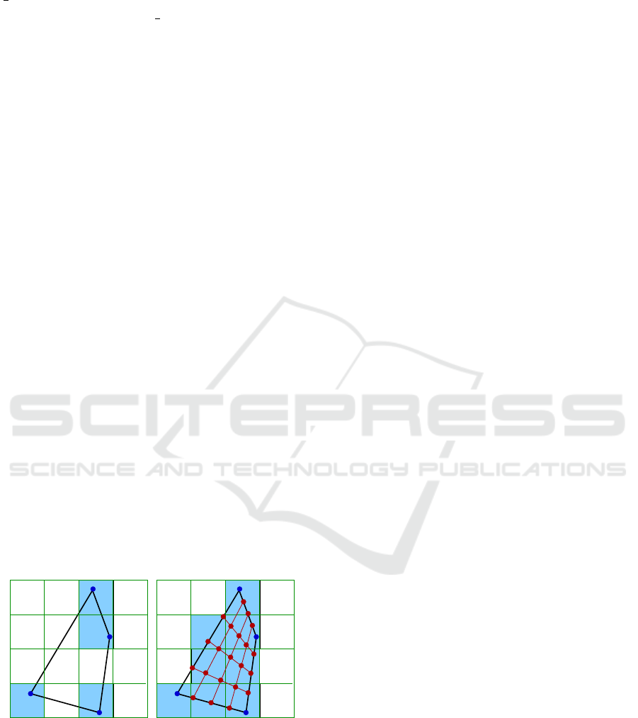
Figure 6 shows the impact of upsampling in the

case of a 2D physical space and a 2D attribute space,

i.e., for a transformed 2D cell with corners a

),...,a

)), u, v ∈ {0,1}, and a histogram

with d = 2 dimensions. Without the upsampling, the

non-empty bins of the histogram are not connected.

After upsampling, the bins between the original non-

empty bins have also been ﬁlled and the 2D cell rep-

resents a continuous region in the 2D attribute space.

Figure 6: Upsampling for a 2D physical space and a 2D

attribute space. Left: The corner points of the 2D cell corre-

spond to bins of the histogram that are not connected. Right:

After upsampling, the ﬁlled bins of the histogram are con-

nected.

When performing the upsampling for all cells of

the volumetric grid, we end up with a histogram,

where all non-empty cells are connected. Hence, we

have overcome the curse of dimensionality. On such a

histogram, we can generate the density-based cluster

hierarchy without the effect of clusters falling apart.

5 ADAPTIVE SCHEME

In order to assure connectivity of non-empty his-

togram bins, we have to upsample in some regions

more than in other regions. As we want to have a

global upsampling rate, some regions may be over-

sampled. Such an oversampling is not a problem in

terms of correctness, but a waste of computation time.

To reduce computation time, we propose to use an

adaptive scheme for upsampling. Since we are deal-

ing with cuboid grid cells, we can adopt an octree

scheme: Starting with an original grid cell, we up-

sample with a factor of two in each dimension. The

original grid cell is partitioned into eight subcells of

equal size. If the corners of a subcell S all corre-

spond to one and the same histogram bin B, i.e., if

uvw

),...,a

uvw

)) fall into the same bin B for

all corners p

uvw

, then we can stop the partitioning S.

If the depth of the octree is d

max

and we stop parti-

tioning S at depth d

stop

, we increase the bin count (or

density, respectively) of bin B by 8

max

−d

stop

. If the

corners of a subcell S do not correspond to the same

histogram bin, we continue with the octree splitting

of S until we reach the maximum octree depth d

max

Memory consumption is another aspect that we

need to take into account, since multivariate volume

data per se are already quite big and we further in-

crease the data volume by applying an upsampling.

However, we can march through each original cell,

perform the upsampling for that cell individually, and

immediately add data point counts to the histogram.

Hence, we never need to store the upsampled version

of the full data. However, we need to store the his-

togram, which can also be substantial as bin sizes are

supposed to be small. We handle the histogram by

storing only non-empty bins in a dynamic data struc-

ture.

6 SHARP MATERIAL

BOUNDARIES

Some data like the ones stemming from medi-

cal imaging techniques may exhibit sharp material

boundaries. It is inappropriate to interpolate across

those boundaries. In practice, such abrupt changes

in attribute values may require our algorithm to exe-

cute many interpolation steps. To avoid interpolation

IVAPP 2018 - International Conference on Information Visualization Theory and Applications

across sharp feature boundaries, we introduce a user-

speciﬁed parameter that deﬁnes sharp boundaries. As

this is directly related to the number of interpolation

steps, the user just decides on the respective maximal

number of interpolation steps d

max

. If two neighbor-

ing points in physical space have attribute values that

lie in histogram cells that would not get connected af-

ter d

max

interpolation steps, we do not perform any in-

terpolation between those points. This is important, as

performing some few interpolation steps across sharp

material boundary may introduce noise artifacts lead-

ing to artiﬁcial new clusters.

7 INTERACTIVE VISUAL

EXPLORATION

After having produced a clustering result of the at-

tribute space that does not suffer from the curse of

dimensionality, it is, of course, of interest to also in-

vestigate the clusters visually in physical and attribute

space. Hence, we want to visualize, which regions in

physical space belong to which attribute space cluster

and what are the values of the respective attributes.

For visualizing the attribute space clusters we

make use of the cluster tree, see Figure 2 (right), and

visualize it in a radial layout, see Figure 8 (lower

row). The cluster tree functions as an interaction wid-

get to select any cluster or any set of clusters. The

properties of the selected clusters can be analyzed us-

ing a linked parallel coordinates plot that shows the

function values in attribute space, see Figure 10 (mid-

dle row).

The distribution of the selected clusters in volume

space can be shown in a respective visualization of

the physical space. We support both a direct volume

rendering approach and a surface rendering approach.

The 3D texture-based direct volume renderer takes

as input only the density values stemming from the

clustering step and the cluster indices, see (Dobrev

et al., 2011). Similarly, we extract boundary surfaces

of the clusters using a standard isosurface extraction

method, see Figure 10 (bottom). We illuminate our

renderings using normals that have been derived as

gradients from the density ﬁeld that stems from the

clustering approach.

8 RESULTS

First, we demonstrate on a simple scalar ﬁeld example

how our approach works and show that the discrete

histogram of interpolated data approaches the contin-

uous analogon as the interpolation depth increases.

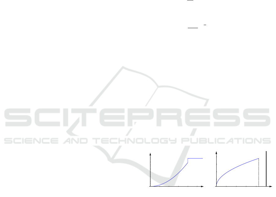
Let scalar ﬁeld f (r) be deﬁned as follows:

f (r) =



for r ≥ 0.8,

1 else,

b = 0.85/0.8

where r stands for the Euclidean distance to the center

of domain [−1,1)

, see Figure 7 (left). The continu-

ous histogram h(x) can be computed using the rela-

tion

h(x)dx =

4π



−1

(r)



, 0 ≤ r ≤ 0.8,

which leads to

h(r) =

4π

3/2

√

r, 0 ≤ r ≤ 0.8.

The continuous histogram is plotted in Fig-

ure 7 (right). The continuous data are clearly

separated into two clusters, which represent the

interior of a sphere and the background in physical

space. However, when sampling the ﬁeld at 30

regular samples in the physical domain. the use of

100 bins in the attribute space leads to the effect

that the sphere cluster breaks into many small parts.

In Figure 8, we demonstrate how our interpolation

approach corrects the histogram (upper row) and the

respective cluster tree (lower row). The resulting

discrete histograms approach the shape of the contin-

uous one as upsampling depth grows. Depth d

max

= 7

is needed to converge to the correct result of the two

clusters.

0.0

0.2

0.4

0.6

0.8

1.0

0.2

0.4

0.6

0.8

1.0

Scalar field

0.0

0.2

0.4

0.6

0.8

1.0

Histogram

Figure 7: Scalar ﬁeld distribution (left) and continuous his-

togram (right) for artiﬁcial data. Bold vertical line denotes

the scaled Dirac function in the histogram.

Second, we design a volumetric multi-attribute

data set, for which the ground truth is known, show

how the size of bins affects the result of the clustering

procedure and demonstrate that interpolation helps to

resolve the issue. Given physical domain [−1; 1)

, we

use the following algebraic surfaces

(x,y,z) = x

−y

−5z = 0, (1)

(x,y,z) = x

+ y

+ (z −1)z

= 0, (2)

see Figure 9 (left). We construct the distributions of

two attributes as functions of algebraic distances to

the surfaces above, i.e.,

= f

(x,y,z)), i = 1, . ..,2.

Overcoming the Curse of Dimensionality When Clustering Multivariate Volume Data

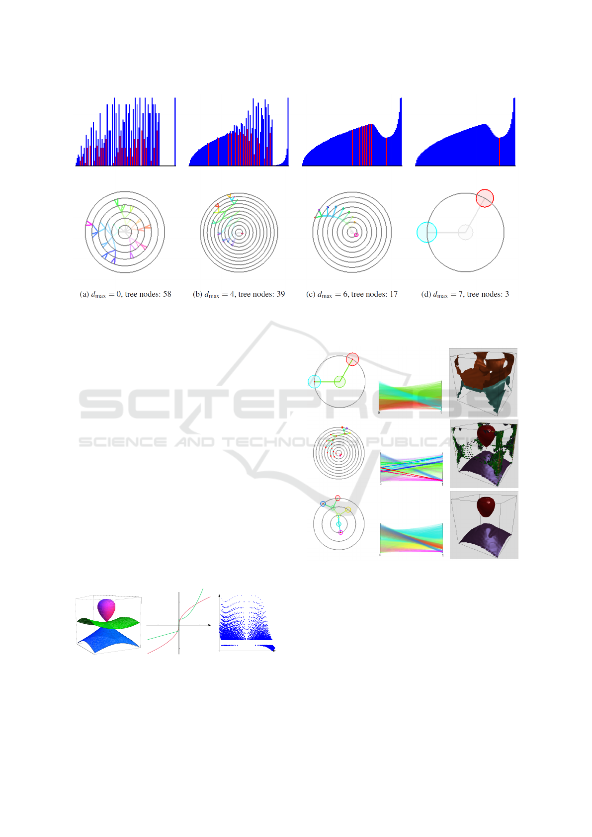
Figure 8: Discrete histograms with 100 bins each and cluster trees at different interpolation depth for data in Figure 7. Red

bins are local minima corresponding to branching in trees. Interpolation makes histograms approach the form of continuous

distribution and corrects cluster tree.

Functions f

are chosen to have a discontinuity or a

large derivative at the origin, respectively, see Fig-

ure 9 (middle). Thus, the surfaces F

are cluster

boundaries in the physical space. The distribution

of the attribute values f

is shown in a 2D scatter-

plot in Figure 9 (right) when sampling over a regular

grid with 50

nodes. The data represent four clus-

ters. Using 10 bins for each attribute to generate the

histogram is not enough to separate all clusters result-

ing in a cluster tree with only 2 clusters as shown in

Figure 10 (upper row). A larger number of bins is

necessary. When increasing the number of bins to 30

for each attribute clusters fall apart due to the curse

of dimensionality, which leads to a noisy result with

too many clusters, see Figure 10 (middle row). How-

ever, applying four interpolation steps ﬁxes the his-

togram. Then, the cluster tree has the desired four

leaves and the boundary for all four clusters are cor-

rectly detected in physical space, see Figure 10 (lower

row).

- 1

Figure 9: Designing a synthetic dataset: Algebraic surfaces

separate clusters in physical space (left). Functions of al-

gebraic distance to the surfaces (middle) deﬁne distribution

of two attributes. The resulting distribution in the attribute

space in form of a 2D scatterplot (right).

Figure 10: Effect of bin size choice and interpolation pro-

cedure on synthetic data with known ground truth. 10

bins

are not enough to separate all clusters resulting in a degen-

erate tree (upper row). 30

bins are too many to keep clus-

ters together (middle row). Interpolation of data with the

same number of bins corrects the tree (lower row). Cluster

trees, parallel coordinates, and clusters in physical space are

shown in the left, mid, and right columns, correspondingly.

Matching colors are used in the coordinated views to allow

for analyzing correspondences.

Next, we apply our methods to the simulation-

based dataset provided in the 2008 IEEE Visualiza-

tion Design Contest (Whalen and Norman, 2008) and

quantify the gain of (modiﬁed) adaptive upsampling.

IVAPP 2018 - International Conference on Information Visualization Theory and Applications

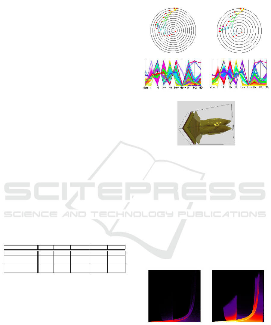
We picked time slice 75 of this ionization front in-

stability simulation. We considered the 10 scalar

ﬁelds (mass density, temperature, and mass fractions

of various chemical elements). What is of interest

in this dataset are the different regions of the transi-

tion phases between atoms and ions of hydrogen (H)

and helium (He). To reduce computational efforts,

we made use of the symmetry of the data with re-

spect to the y = 124 and the z = 124 planes and re-

stricted consideration to data between x = 275 and

x = 500 localizing the front. When applying the clus-

tering approach to the original attribute space using

a 10-dimensional histogram with 10 bins in each di-

mension, we obtain a cluster tree with 15 mode clus-

ters. The cluster tree and the corresponding paral-

lel coordinates plot are shown in Figure 11(a). Not

all of the clusters are meaningful and some of them

should have been merged to a single cluster. These

mode clusters are not clearly separated when observ-

ing the parallel coordinates plot. After applying our

approach with d

max

= 5, such clusters were merged

leading to 12 modes and a simpliﬁed cluster tree. Re-

sults are shown in Figure 11(b). The timings of adap-

tive and non-adaptive upsampling for different inter-

polation depths are given in Table 1. “Modiﬁed adap-

tive” upsampling refers to the approach with no up-

sampling across sharp material boundaries, see Sec-

tion sec:sharp. The adaptive schemes lead to a signif-

icant speed up (up to one order of magnitude). All nu-

merical tests presented in this section were performed

on a PC with an Intel Xeon 3.20GHz processor.

Table 1: Computation times for non-adaptive vs. adaptive

upsampling scheme at different upsampling depths (2008

IEEE Visualization Design Contest dataset).

max

0 1 2 3 4

Non-adaptive 7.57s 59.84s 488.18s 3929s 27360s

Adaptive 5.99s 27.5s 136.56s 717.04s 3646s

Non-empty bins 1984 3949 6400 9411 12861

Modiﬁed adaptive 14.3s 26.0s 80.91s 437.76s 2737s

Non-empty bins 1984 2075 2451 3635 5945

Finally, we demonstrate that scatterplots of up-

sampled data approach the quality of continu-

ous scatterplots as presented by Bachthaler and

Weiskopf (Bachthaler and Weiskopf, 2008) and the

follow-up papers. The “tornado” dataset was sam-

pled on a uniform grid of resolution 128

. Similar

to (Bachthaler and Weiskopf, 2008), the magnitude of

the velocity and the velocity in z-direction were taken

as two data dimensions. In Figure 12, we show scat-

terplots of the original data and of the adaptively up-

sampled data with interpolation depth 5. The number

of bins is 300 for each attribute. The quality of the up-

sampled scatterplot is similar to the continuous scat-

terplot presented in (Bachthaler and Weiskopf, 2008).

We would like to note that rigorously speeking, eval-

(a) d

max

= 0, modes: 15 (b) d

max

= 5, modes: 12

Figure 11: Cluster tree (upper row), parallel coordinates

plot (middle row), and physical space visualization (lower

row) for the 2008 IEEE Visualization Design Contest data

set, time slice 75, for original attribute space using a 10-

dimensional histogram (a) before and (b) after interpolation.

Several mode clusters are merged when applying our ap-

proach, which leads to a simpliﬁcation of the tree and better

cluster separation. Matching colors are used in the coordi-

nated views to allow for analyzing correspondences.

uation of vector magnitude and interpolation are not

commutative operations. Thus, the upsampling with

respect to the ﬁrst chosen parameter could have sig-

niﬁcant errors in both the continuous and the discrete

setting. However, we intentionally followed this way

to be able to compare our results with results pre-

sented in (Bachthaler and Weiskopf, 2008).

Figure 12: Scatterplots of the “tornado” dataset initially

sampled on 128

regular grid. Original data (left) and result

of adaptive upsampling with interpolation depth 5 (right)

are shown.

Overcoming the Curse of Dimensionality When Clustering Multivariate Volume Data

9 DISCUSSION

Histogram Bin Size. The size of the bins of the his-

togram can be chosen arbitrarily. Of course, smaller

bin sizes produce better results, as they can resolve

better the shape of the clusters. Too large bin sizes

lead to an improper merging of clusters. In terms of

clustering quality, bin sizes can be chosen arbitrar-

ily small, as very small bin sizes do not affect the

clustering result negatively. However, storing a high-

dimensional histogram with small bin sizes can be-

come an issue. Our current implementation stores the

histogram in main memory, which limits the bin sizes

we can currently handle. This in-core solution allows

us to produce decent results, as we are only storing

non-empty bins. Nevertheless, for future work, it may

still be desirable to implement an out-of-core version

of the histogram generation. This can be achieved

by splitting the histogram into parts and only storing

those parts. However, an out-of-core solution would

negatively affect the computation times. Also, the

smaller the bin sizes, the more upsampling is neces-

sary.

Upsampling Rate. The upsampling rate is inﬂu-

enced by the local variation in the values of the multi-

variate ﬁeld and the bin size of the histogram. Let s

bin

be the bin size of the histogram. Then, an upsampling

may be necessary, if two data points in attribute space

are more than distance s

bin

apart. As the upsampling

rate is deﬁned globally, it is determined by the largest

variation within a grid cell. Let s

data

is the maximum

distance in attribute space between two data points,

whose corresponding points in physical space belong

to one grid cell. Then, the upsampling rate shall be

larger than

data

bin

. This ratio refers to the upsampling

rate per physical dimension.

When using the adaptive scheme presented in Sec-

tion 5, the upsampling rate per dimension is always

a power of two. When a sufﬁciently high upsam-

pling rate has been chosen, the additional computa-

tions when upsampling with the next-higher power of

two in the adaptive scheme are modest, as computa-

tions for most branches of the octree have already ter-

minated.

10 CONCLUSION

We presented an approach for multivariate volume

data visualization that is based on clustering the

multi-dimensional attribute space. We overcome the

curse of dimensionality by upsampling the attribute

space according to the neighborhood relationship in

physical space. Trilinear interpolation is applied

to the attribute vectors to generate multidimensional

histograms, where the support, i.e., all non-empty

bins, is a connected component. Consequently, the

histogram-based clustering does not suffer from clus-

ters falling apart when using small bin sizes. We ap-

ply a hierarchical clustering method that generates a

cluster tree without having to pick density thresholds

manually or heuristically. In addition to a cluster tree

rendering, the clustering results are visualized using

coordinated views to parallel coordinates for an at-

tribute space rendering and to physical space render-

ing. The coordinated views allows for a comprehen-

sive analysis of the clustering result.

ACKNOWLEDGMENTS

This work was supported by the Deutsche

Forschungsgemeinschaft (DFG) under project

grant LI 1530/6-2.

REFERENCES

(2010). Competition data set and description.

2010 IEEE Visualization Design Contest,

http://viscontest.sdsc.edu/2010/.

Akiba, H. and Ma, K.-L. (2007). A tri-space visualization

interface for analyzing time-varying multivariate vol-

ume data. In In Proceedings of Eurographics/IEEE

VGTC Symposium on Visualization, pages 115–122.

Ankerst, M., Breunig, M. M., Kriegel, H.-P., and Sander, J.

(1999). Optics: ordering points to identify the clus-

tering structure. In Proceedings of the 1999 ACM

SIGMOD international conference on Management of

data, pages 49 – 60.

Bachthaler, S. and Weiskopf, D. (2008). Continuous scatter-

plots. IEEE Transactions on Visualization and Com-

puter Graphics (Proceedings Visualization / Informa-

tion Visualization 2008), 14(6):1428–1435.

Bachthaler, S. and Weiskopf, D. (2009). Efﬁcient and adap-

tive rendering of 2-d continuous scatterplots. Com-

puter Graphics Forum (Proc. Eurovis 09), 28(3):743

– 750.

Bellman, R. E. (1957). Dynamic programming. Princeton

University Press.

Blaas, J., Botha, C. P., and Post, F. H. (2007). Interactive

visualization of multi-ﬁeld medical data using linked

physical and feature-space views. In EuroVis, pages

123–130.

Daniels II, J., Anderson, E. W., Nonato, L. G., and Silva,

C. T. (2010). Interactive vector ﬁeld feature identiﬁ-

cation. IEEE Transactions on Visualization and Com-

puter Graphics, 16:1560–1568.

IVAPP 2018 - International Conference on Information Visualization Theory and Applications

Dobrev, P., Long, T. V., and Linsen, L. (2011). A cluster

hierarchy-based volume rendering approach for inter-

active visual exploration of multi-variate volume data.

In Proceedings of 16th International Workshop on Vi-

sion, Modeling and Visualization (VMV 2011), pages

137–144. Eurographics Association.

Ester, M., Kriegel, H.-P., Sander, J., and Xu, X. (1996).

A density-based algorithm for discovering clusters in

large spatial databases with noise. In Proceedings of

the second international conference on knowledge dis-

covery and data mining, page 226231.

Han, J. and Kamber, M. (2006). Data Mining: Concepts

and Techniques. Morgan Kaufmann Publishers.

Hartigan, J. A. (1975). Clustering Algorithms. Wiley.

Hartigan, J. A. (1985). Statistical theory in clustering. Jour-

nal of Classiﬁcation, 2:62–76.

Heinrich, J., Bachthaler, S., and Weiskopf, D. (2011). Pro-

gressive splatting of continuous scatterplots and par-

allel coordinates. Comput. Graph. Forum, 30(3):653–

662.

Hinneburg, A. and Keim, D. (1998). An efﬁcient approach

to clustering in large multimedia databases with noise.

In Proceedings of the fourth international conference

on knowledge discovery and data mining, page 5865.

Hinneburg, A., Keim, D. A., and Wawryniuk, M. (1999).

Hd-eye: Visual mining of high-dimensional data.

IEEE Computer Graphics and Applications, pages

22–31.

Jain, A. K. and Dubes, R. C. (1988). Algorithms for Clus-

tering Data. Prentice Hall.

anicke, H., Wiebel, A., Scheuermann, G., and Kollmann,

W. (2007). Multiﬁeld visualization using local statis-

tical complexity. IEEE Transaction on Visualization

and Computer Graphics, 13(6):1384–1391.

Karypis, G., Han, E. H., and Kumar, V. (1999). Chameleon:

Hierarchical clustering using dynamic modeling.

Computer, 32(8):68–75.

Lehmann, D. J. and Theisel, H. (2010). Discontinuities in

continuous scatter plots. IEEE Transactions on Visu-

alization and Computer Graphics, 16:1291–1300.

Lehmann, D. J. and Theisel, H. (2011). Features in continu-

ous parallel coordinates. Visualization and Computer

Graphics, IEEE Transactions on, 17(12):1912 –1921.

Linsen, L., Long, T. V., and Rosenthal, P. (2009). Link-

ing multi-dimensional feature space cluster visual-

ization to surface extraction from multi-ﬁeld volume

data. IEEE Computer Graphics and Applications,

29(3):85–89. linsenlongrosenthalvcgl.

Linsen, L., Long, T. V., Rosenthal, P., and Rosswog, S.

(2008). Surface extraction from multi-ﬁeld particle

volume data using multi-dimensional cluster visual-

ization. IEEE Transactions on Visualization and Com-

puter Graphics, 14(6):1483–1490. linsenlongrosen-

thalrosswogvcglsmoothvis.

Long, T. V. (2009). Visualizing High-density Clusters in

Multidimensional Data. PhD thesis, School of Engi-

neering and Science, Jacobs University, Bremen, Ger-

many.

Maciejewski, R., Woo, I., Chen, W., and Ebert, D. (2009).

Structuring feature space: A non-parametric method

for volumetric transfer function generation. IEEE

Transactions on Visualization and Computer Graph-

ics, 15:1473–1480.

Oeltze, S., Doleisch, H., Hauser, H., Muigg, P., and Preim,

B. (2007). Interactive visual analysis of perfusion

data. IEEE Transaction on Visualization and Com-

puter Graphics, 13(6):1392–1399.

Sauber, N., Theisel, H., and Seidel, H.-P. (2006). Multiﬁeld-

graphs: An approach to visualizing correlations in

multiﬁeld scalar data. IEEE Transactions on Visual-

ization and Computer Graphics, 12(5):917–924.

Stuetzle, W. (2003). Estimating the cluster tree of a density

by analyzing the minimal spanning tree of a sample.

Journal of Classiﬁcation, 20:25–47.

Stuetzle, W. and Nugent, R. (2007). A generalized single

linkage method for estimating the cluster tree of a den-

sity. Technical Report.

Whalen, D. and Norman, M. L. (2008). Com-

petition data set and description. 2008

IEEE Visualization Design Contest,

http://vis.computer.org/VisWeek2008/vis/contests.html.

Wong, A. and Lane, T. (1983). A kth nearest neighbor clus-

tering procedure. Journal of the Royal Statistical So-

ciety, Series B, 45:362–368.

Woodring, J. and Shen, H.-W. (2006). Multi-variate, time

varying, and comparative visualization with contex-

tual cues. IEEE Transactions on Visualization and

Computer Graphics, 12(5):909–916.

Overcoming the Curse of Dimensionality When Clustering Multivariate Volume Data