Opponent Modelling in the Game of Tron using Reinforcement Learning
Stefan J. L. Knegt
1
, Madalina M. Drugan
2
and Marco A. Wiering
1
1
Institute of Artificial Intelligence and Cognitive Engineering, University of Groningen, The Netherlands
2
ITLearns.Online, The Netherlands
Keywords:
Reinforcement Learning, Opponent Modelling, Q-learning, Computer Games.
Abstract:
In this paper we propose the use of vision grids as state representation to learn to play the game Tron using
neural networks and reinforcement learning. This approach speeds up learning by significantly reducing the
number of unique states. Furthermore, we introduce a novel opponent modelling technique, which is used to
predict the opponent’s next move. The learned model of the opponent is subsequently used in Monte-Carlo
roll-outs, in which the game is simulated n-steps ahead in order to determine the expected value of conducting a
certain action. Finally, we compare the performance using two different activation functions in the multi-layer
perceptron, namely the sigmoid and exponential linear unit (Elu). The results show that the Elu activation
function outperforms the sigmoid activation function in most cases. Furthermore, vision grids significantly
increase learning speed and in most cases this also increases the agent’s performance compared to when the
full grid is used as state representation. Finally, the opponent modelling technique allows the agent to learn
a predictive model of the opponent’s actions, which in combination with Monte-Carlo roll-outs significantly
increases the agent’s performance.
1 INTRODUCTION
Reinforcement learning algorithms allow an agent to
learn from its environment and thereby optimise its
behaviour (Sutton and Barto, 1998). Such environ-
ments can be modelled as a Markov Decision Pro-
cess (MDP) (van Otterlo and Wiering, 2012; Bell-
man, 1957), where an agent tries to learn an op-
timal policy from trial and error. Reinforcement
learning algorithms have been widely applied in the
area of games. A well-known example is backgam-
mon (Tesauro, 1995), where reinforcement learning
has led to great success. This paper examines the ef-
fectiveness of reinforcement learning for the game of
Tron. One of the main challenges of using reinforce-
ment learning in games is the large size of the state
space. Another challenge is how an agent can learn to
model its opponent effectively and use this opponent’s
model to significantly increase its performance.
To deal with large state spaces, in many cases
the agent is constructed using a multi-layer percep-
tron (MLP) (Rumelhart et al., 1988). The MLP will
receive the current game state as its input and has
to determine the move that will result in the high-
est reward in the long term. The combination of an
MLP and reinforcement learning has showed promis-
ing results, for instance in Backgammon (Tesauro,
1995), Ms. PacMan (Bom et al., 2013) and Star-
craft (Shantia et al., 2011). Furthermore, deep rein-
forcement learning using neural networks with many
layers have also obtained impressive results on a vari-
ety of games (Mnih et al., 2013).
In most research on learning to play games with
connectionist reinforcement learning, the MLP uses
only the well-known sigmoid activation function.
However, there are other choices such as the expo-
nential linear unit (Elu). The exponential linear unit
has three advantages compared to the sigmoid func-
tion (Clevert et al., 2015). It alleviates the vanishing
gradient problem by its identity for positive values,
it can return negative values which might improve
learning, and it is better able to deal with a large num-
ber of inputs. This activation function has shown to
outperform the ReLU in a convolutional neural net-
work on the ImageNet dataset (Clevert et al., 2015).
Another way to deal with large state spaces is to give
the agent a partial view of the environment. If we
look at how humans play the game Tron we see that
they mainly focus their attention around the current
position of the agent. Therefore, vision grids (Shan-
tia et al., 2011) can be useful. A vision grid can be
seen as a snapshot of the environment from the agent’s
point of view. An example could be a three by three
square around the ’head’ of the agent. By using a
Knegt, S., Drugan, M. and Wiering, M.
Opponent Modelling in the Game of Tron using Reinforcement Learning.
DOI: 10.5220/0006536300290040
In Proceedings of the 10th International Conference on Agents and Artificial Intelligence (ICAART 2018) - Volume 2, pages 29-40
ISBN: 978-989-758-275-2
Copyright © 2018 by SCITEPRESS – Science and Technology Publications, Lda. All rights reserved
29

vision grid of an appropriate size, the agent can ac-
quire the most important information about the dy-
namic state of the environment. Not only does this
dramatically decrease the number of unique states,
it also reduces the amount of irrelevant information,
which can speed up the learning process of the agent.
For most game research, the agent does not learn
an explicit opponent model. In most cases, roll-outs
or lookahead strategies are used that select opponent’s
actions according to how the agent itself would se-
lect actions or according to simple rules. Although
roll-outs have shown to substantially increase per-
formance in games such as Backgammon (Tesauro
and Galperin, 1997), Go (Bouzy and Helmstetter,
2004; Silver et al., 2016a), and Scrabble (Shep-
pard, 2002), the disadvantage of this approach is
that particular weaknesses of the opponent cannot
be exploited, as no true model of how the oppo-
nent selects actions is used. Opponent modelling has
been studied for imperfect-information games such as
poker (Ganzfried and Sandholm, 2011; Southey et al.,
2005). Furthermore, in combination with Q-learning
(Watkins and Dayan, 1992) it has proven to lead to
better performances (He et al., 2016). However, as
noted by (Collins, 2007), the learned models are often
environment specific and take considerable effort to
learn. As a solution to this problem, Mealing (Meal-
ing, 2015) proposed a dynamic opponent modelling
variant, which uses sequence prediction to learn high
rewarding strategies.
Contributions: In this paper, we developed differ-
ent state representations for the game of Tron. We
show that with vision grids we can reduce the number
of unique states, which helps overcoming the chal-
lenge of using reinforcement learning in problems
with large state spaces. We use the information from
the vision grids as input for a multi-layer perceptron
that is trained using a reinforcement learning algo-
rithm. Next to using the common sigmoid function in
the hidden layer of the MLP, we will also use the Elu
activation function and compare the results of both
activation functions. The most important contribution
of this paper is a novel opponent modelling technique.
In our proposed algorithm, the agent learns the oppo-
nent’s behaviour by predicting the next move of the
opponent, observing the result, and adjusting the neu-
ral network’s parameters based on this observation. If
the opponent is following a policy, the agent should
be able to learn this policy over time. This model
of the opponent is subsequently used in Monte-Carlo
roll-outs. In such a roll-out the game is simulated n
steps ahead in order to determine the expected value
of performing action a in state s and subsequently ex-
ecuting the action that is associated with the highest
Q-value in each state. In these roll-outs, the learned
opponent model is used to select actions for the oppo-
nent. The roll-outs are performed multiple times and
the results are averaged. We performed many differ-
ent experiments to compare all methods (3 state rep-
resentations, sigmoid / Elu, opponent model / no op-
ponent model, different numbers of roll-outs). From
the results we can conclude that vision grids are effec-
tive for faster training and better final performances.
Furthermore, when we combine the vision grids with
opponent modelling and roll-outs, the performances
are very good, reaching very high scores against 2 dif-
ferent fixed opponents.
Outline: In the next section we explain the frame-
work that was built to simulate the game and agent.
Section 3 describes reinforcement learning combined
with multi-layer perceptrons. In Section 4, we explain
the use of vision grids for Tron and the novel oppo-
nent modelling technique. Then in section 5 we de-
scribe the experiments and show their results. Finally,
in section 6 we present our conclusions and possible
future work.
2 THE GAME OF TRON
Tron is an arcade video game released in 1982 and
was inspired by the Walt Disney motion picture Tron.
In this game the player guides a light cycle in an arena
against an opponent. The player has to do this, while
avoiding the walls and the trails of light left behind
by the opponent and player itself. See Figure 1 for
a graphical depiction of the game. We developed a
framework that implements the game of Tron as a se-
quential decision problem where each agent selects
an action for each new game state. In this research
the game is played with two players. The environ-
ment is represented by a 10 by 10 grid in which the
player starts at a random location in the top half of
the grid and the opponent in the bottom half. After
that, both players decide on an action to carry out.
The action space consists of the four directions the
agents can move in. When the action selection phase
is completed, both actions get carried out and the new
game state is evaluated. In case both agents move to
the same location, the game ends in a draw. A player
loses if it moves to a location that is previously vis-
ited by either itself or the opponent or when the agent
wants to move to a location outside of the grid. If
it happens that both agents lose at the same moment,
the game counts as a draw. We estimate the number
of possible different states in the game to be of the
order 10
20
, which is similar to the game Othello that
consists of a board of 7 × 7 cells.
ICAART 2018 - 10th International Conference on Agents and Artificial Intelligence
30

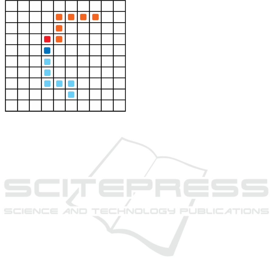
Figure 1: Tron game environment with two agents, where
their heads or current location are in a darker colour.
For the opponent we used two different imple-
mentations. Both fixed opponents always first check
whether their intended move is possible and therefore
will never lose unless they are fully enclosed. The
first agent randomly chooses an action from the pos-
sible actions, while the second agent always tries to
execute its previous action again. If this is not pos-
sible, the opponent randomly chooses an action that
is possible and keeps repeating that action. This im-
plies that this opponent only changes its action when
it encounters a wall, the opponent or its own tail. This
strategy is very effective in the game of Tron, because
it is very efficient in the use of free space and it makes
the agent less likely to enclose itself. We tested these
opponents by letting them play against each other,
and observed that the opponent employing the strat-
egy of going straight as long as possible only loses
25% of the games and 20% of the games end in a
draw. From here on we will refer to the agent em-
ploying the collision-avoiding random policy as the
random opponent and the other opponent will be re-
ferred to as the semi-deterministic opponent.
3 REINFORCEMENT LEARNING
When the agent starts playing the game, it will ran-
domly choose actions from its action space. In or-
der to improve its performance, the agent has to learn
the best action in a given game state and therefore we
train the agent using reinforcement learning. Rein-
forcement learning is a learning method in which the
agent learns to select the optimal action based on in-
game rewards. Whenever the agent loses a game it re-
ceives a negative reward or punishment and if it wins
it will receive a positive reward. As it plays a large
number of games, the agent should learn to select the
action that leads to the highest possible expected re-
ward given the current game state. Reinforcement
learning techniques are often applied to environments
that can be modelled as a so-called Markov Decision
Process (MDP) (Bellman, 1957). An MDP is defined
by the following components:
• A finite set of states S, where s
t
∈ S is the state at
time t.
• A finite set of actions A, where a
t
∈ A is the action
executed at time t.
• A transition function T (s, a,s
0
). This function
specifies the probability of ending up in state s
0
after executing action a in state s. Whenever the
environment is fully deterministic, we can ignore
the transition probability. This is not the case in
the game of Tron, since it is played against an op-
ponent for which we cannot perfectly anticipate
its next move.
• A reward function R(s, a,s
0
), which specifies the
reward for executing action a in state s and sub-
sequently going to state s
0
. In our framework, the
reward is equal to 1 for a win, 0 for a draw, and
−1 in case the agent loses. Note that there are no
intermediate rewards.
• A discount factor γ to discount future rewards,
where 0 ≤ γ ≤ 1.
To let the agent act in this MDP, we need a map-
ping from states to actions. This is given by the pol-
icy π(s), which returns for any state s the action to
perform. The value of a policy is given by the sum
of the discounted future rewards starting in a state s
following the policy π:
V
π
(s) = E

∞
∑
t=0
γ
t
r
t
|s
0
= s,π

(1)
Where r
t
is the reward received at time t. The
value function gives the expected outcome of the
game if both players select the actions given by their
policy. The value of a state is the long-term reward the
agent will receive, while the reward of a state is only
short-term. Therefore, the agent has to choose the
state with the highest possible value. We can rewrite
equation 1 in terms of the components of an MDP:
V
π
(s) =
∑
s
0
T (s,π(s),s
0
)(R(s,π(s),s
0
) + γ V
π
(s
0
))
(2)
From equation 2 we see that the value of a particu-
lar state s depends on the transition function, the prob-
ability of going to state s
0
times the reward obtained in
this new state s
0
and the value of the next state times
Opponent Modelling in the Game of Tron using Reinforcement Learning
31

the discount factor. In practice, the transition function
is often unknown and therefore we have to use a rein-
forcement learning algorithm. Next, we will look at the
particular reinforcement learning algorithm employed in
this research: Q-learning.
3.1 Q-learning
In this research we will be using Q-learning (Watkins
and Dayan, 1992), for which the value of a state becomes
a Q-value of a state-action pair, Q(s,a), which gives the
value of performing action a in state s. This Q-value for
a given policy is given by equation 3.
Q
π
(s,a) = E

∞
∑
t=0
γ
t
r
t
|s
0
= s, a
0
= a, π

(3)
The value of performing action a in state s is the ex-
pected sum of the discounted future rewards following
policy π. The Q-value of an individual state-action pair
is given by:
Q(s
t
,a
t
) = E(r
t
) + γ
∑
s
t+1
T (s
t
,a
t
,s
t+1
)max
a
Q(s
t+1
,a) (4)
The Q-value of a state-action pair depends on the ex-
pected reward and the highest Q-value in the next state.
However, we do not know s
t+1
as it depends on the action
of the opponent. Therefore, Q-learning keeps a running
average of the Q-value of a certain state-action pair. The
Q-learning algorithm is given by:
b
Q(s
t
,a
t
) ←
b
Q(s
t
,a
t
)+α(r
t
+γ max
a
b
Q(s
t+1
,a)−
b
Q(s
t
,a
t
))
Where 0 ≤ α ≤ 1 denotes the learning rate. As we en-
counter the same state-action pair multiple times, we up-
date the Q-value to find the average Q-value of this state-
action pair. This kind of learning is called temporal-
difference learning (Sutton, 1988).
3.2 Function Approximator
Whenever the state space is relatively small, one can eas-
ily store the Q-values for all state-action pairs in a lookup
table. However, since the state space in the game of Tron
is far from small the use of a lookup table is not feasible
in this research. In addition, since there are many differ-
ent states it could happen that even after training, some
states have not been encountered before. When a state
has not been encountered before, action selection hap-
pens without information from experience. Therefore,
we use a neural network as function approximator. To
be more precise, we will be using a multi-layer percep-
tron (MLP) to estimate Q(s,a). This MLP will receive
as input the current game state s and its output will be the
Q-value for each action given the input state. One could
also choose to use four different MLPs, which output one
Q-value each (one for every action). We have tested both
set-ups and there was a small advantage of using a sin-
gle action neural network. The neural network is trained
using back-propagation (Rumelhart et al., 1988), where
the target Q-value is calculated using equation 5. As a
simplification we set the learning rate α in this equa-
tion equal to 1, because the back-propagation algorithm
of the neural network already contains a learning rate,
which controls for the speed of learning. The target Q-
value for action a
t
in state s
t
is therefore:
Q
target
(s
t
,a
t
) ← r
t
+ γmax
a
b
Q(s
t+1
,a) (5)
This target is valid as long as the action taken in the state-
action pair does not result in the end of the game. When-
ever that is the case, the target Q-value is equal to the
first term of the right-hand side of equation 5, the reward
received in the final game:
Q
target
(s
t
,a
t
) ← r
t
(6)
3.2.1 Activation Function
In order to allow the neural network’s value function ap-
proximation to be non-linear we use an activation func-
tion in the hidden layer. One of the most often used acti-
vation functions is the sigmoid function:
O(a) =
1
1 + e
−a
(7)
This function transforms the weighted sum of inputs for
a hidden unit to a value between 0 and 1. Recently, it has
been proposed that the exponential linear unit performs
better in some domains (Clevert et al., 2015). We will
compare the performance of the agent using the sigmoid
function and the exponential linear unit (Elu) in the hid-
den layer. The exponential linear unit is given by the
following equation:
O(a) =

a if a ≥ 0
β(e
a
− 1) if a < 0
(8)
We set β equal to 0.01 after some preliminary experi-
ments. This function transforms negative activations to
a small negative value, while positive activation is unaf-
fected. We will compare the performance of the agent
with both activation functions to determine which per-
forms better for learning to play Tron.
4 STATE REPRESENTATION AND
OPPONENT MODELS
In this section, we will first describe the different state
representations that will be used by the agent. Then,
we will describe how a model of the opponent can be
learned and used for selecting actions using roll-outs.
ICAART 2018 - 10th International Conference on Agents and Artificial Intelligence
32

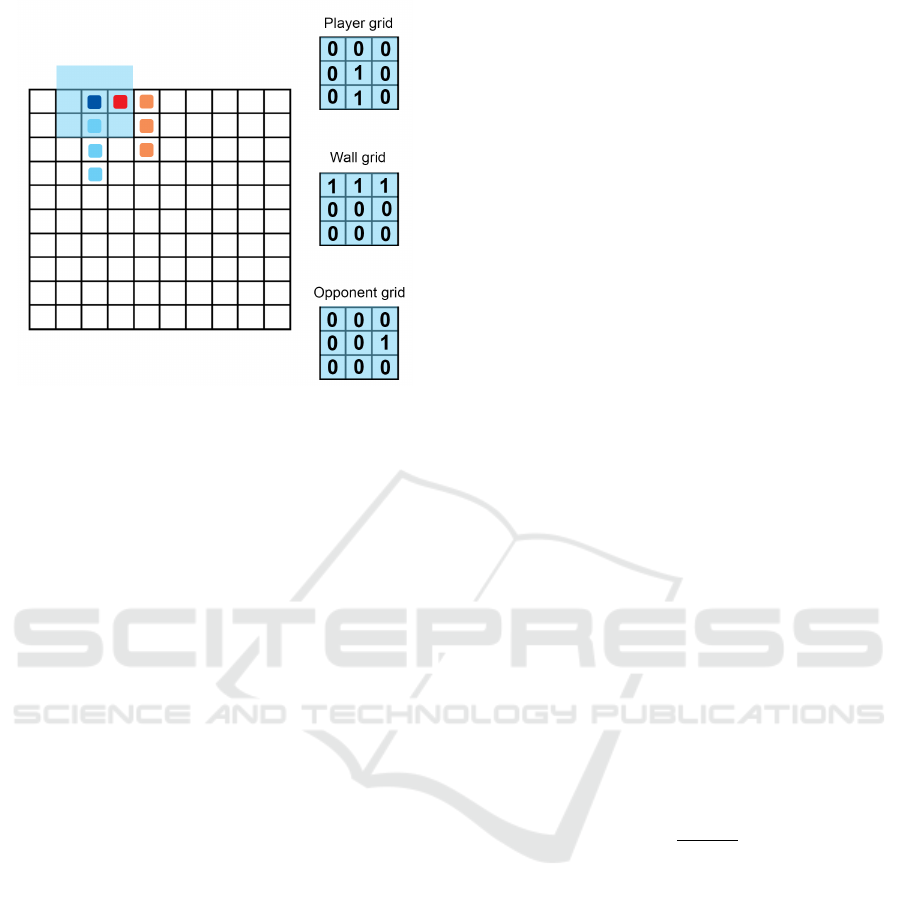
Figure 2: Vision grid example with the current location of
both players in a darker color.
4.1 Vision Grids
The first state representation used as input to the MLP
is the entire game grid (10 × 10). This translates to 100
input nodes, which have a value of one whenever it is
visited by one of the agents and zero otherwise. Another
10 by 10 grid is fed into the network, but this time only
the current position of the agent has a value of one. This
input allows the agent to know its own current position
within the environment. The second type of state rep-
resentation and input to the MLP that will be tested are
vision grids. A vision grid can be seen as a snapshot
of the environment taken from the point of view of the
agent. This translates to a square grid with an uneven
dimension centred around the head of the agent. To re-
ceive the most relevant information from the state of the
game, three different types of vision grids are combined
(in all these grids the standard value is zero):
• The player grid contains information about the loca-
tions visited by the agent itself: whenever the agent
has visited the location it will have a value of one
instead of zero.
• The opponent grid contains information about the lo-
cations visited by the opponent: if the opponent is in
the ’visual field’ of the agent these locations are en-
coded with a one.
• The wall grid represents the walls: whenever the
agent is close to a wall the wall locations will get
a value of one.
An example game state and the three associated vision
grids can be found in Figure 2. We will test vision grids
with a size of three by three (small vision grids) and five
by five (large vision grids) and compare the performance
of the agents with these small and large vision grids to an
agent that receives all information from the game state.
4.2 Opponent Modelling
This paper introduces an opponent modelling technique
with which a model of the opponent is learned from ob-
servations. This model can subsequently be used in plan-
ning algorithms such as Monte-Carlo roll-outs. Planning
is one of the key challenges of artificial intelligence (Sil-
ver et al., 2016b). Many opponent modelling techniques
focus on probabilistic models and imperfect-information
games (Southey et al., 2005; Ganzfried and Sandholm,
2011), which makes them very problem specific. Our
novel opponent modelling technique predicts the oppo-
nent’s action using the multi-layer perceptron and learns
from the observed actions using the back-propagation al-
gorithm (Rumelhart et al., 1988). Over time the agent
learns to model which action the opponent will likely
select when it is in a specific state. The model is a prob-
ability distribution of the opponent’s next move given the
state representation. Because of its simplicity, this tech-
nique can be generalised to any setting in which the op-
ponent’s actions are observable. Another benefit of this
technique is that the agent simultaneously learns a policy
and a model of the opponent, which means that no extra
phase is needed for the learning process. In addition,
the opponent modelling happens with the same neural
network that calculates the Q-values for the agent. This
might allow the agent to learn hidden features regarding
the opponent’s behaviour, which could further increase
performance.
For modelling the opponent, four output nodes are
appended to the network, which represent the probabil-
ity distribution over the opponent’s possible actions. The
output can be interpreted as a probability distribution,
because we use a softmax layer over the four appended
output nodes. The softmax function transforms the vec-
tor o containing the output modelling values for the next
K = 4 possible actions of the opponent to values in the
range [0,1] that add up to one:
P(s
t
,o
i
) =
e
o
i
∑
K
k=1
e
o
k
(9)
This transforms the output values to the probability of
the opponent conducting action o
i
in state s
t
. In addition
to these four extra output nodes, the state representation
for the neural network changes when modelling the op-
ponent. In the case of the standard input representation
by the full grid, an extra grid is added where the head
of the opponent has a value of one. In the case of vi-
sion grids, an extra 4 vision grids are constructed. The
first three are the same as before, but then from the op-
ponent’s point of view. In addition, an opponent-head
grid is constructed which contains information about the
current location of the head of the opponent. If the op-
ponent’s head is in the agent’s visual field, this location
will be encoded with a one.
In order to learn the opponent’s policy, the network
is trained using back-propagation where the target vec-
tor is one for the action taken by the opponent and zero
for all other actions. If the opponent is following a de-
terministic policy, this allows the agent to perfectly fore-
Opponent Modelling in the Game of Tron using Reinforcement Learning
33

cast the opponent’s next move after sufficient training.
Although in reality a policy is seldom entirely determin-
istic, players use certain rules to play a game. Therefore,
our semi-deterministic agent is a perfect example to test
opponent modelling against.
Once the agent has learned the opponent’s policy,
its prediction about the opponent’s next move will be
used in so-called Monte Carlo roll-outs (Tesauro and
Galperin, 1997). Such a roll-out is used to estimate the
value Q
sim
(s,a), the expected Q-value of performing ac-
tion a in state s and subsequently performing the action
suggested by the current policy for n − 1 steps. The op-
ponent’s actions are selected on the basis of the agent’s
model of the agent. If one roll-out is used the opponent’s
move with the highest probability is carried out. When
more than one roll-out is performed, the opponent’s ac-
tion is selected based on the probability distribution. At
every action selection moment in the game m roll-outs
of length n are performed and the results are averaged.
The expected Q-value is equal to the reward obtained in
the simulated game (1 for winning, 0 for a draw, and -1
for losing) times the discount factor to the power of the
number of moves conducted in this roll-out i:
b
Q
sim
(s
t
,a
t
) = γ
i
r
t+i
(10)
If the game is not finished before reaching the roll-out
horizon the simulated Q-value is equal to the discounted
Q-value of the last action performed:
b
Q
sim
(s
t
,a
t
) = γ
n
b
Q(s
t+n
,a
t+n
) (11)
See algorithm 1 for a detailed description.
This kind of roll-out is also called a truncated roll-
out as the game is not necessarily played to its conclu-
sion (Tesauro and Galperin, 1997). In order to deter-
mine the importance of the number of roll-outs m, we
will compare the performance of the agent with one roll-
out and ten roll-outs.
5 EXPERIMENTS AND RESULTS
To compare the different state representations, the use of
different activation functions in the MLP and the useful-
ness of the opponent modelling technique and roll-outs,
many different experiments have been conducted. In all
experiments the agent is trained for 1.5 million games
against two different opponents, which lasts for around
one day for one simulation. After that, 10,000 test games
are played. In these test games, the agent makes no ex-
plorative actions. In order to obtain meaningful results,
all experiments are conducted ten times and the results
are averaged. The performance is measured as the num-
ber of games won plus 0.5 times the number of games
tied. This number is divided by the number of games to
get a score between 0 and 1. This is a common perfor-
mance score for games.
Algorithm 1 : Monte-Carlo Roll-out with Opponent
Model.
Input: Current game state s
t
, starting action a
t
, hori-
zon N, number of roll-outs M
Output: Average reward of performing action a
t
at
time t and subsequently following the policy over
M roll-outs
for m = 1,2,..M do
i = 0
Perform starting action a
t
if M = 1 then
o
t
← argmax
o
P(s
t
,o)
else if M > 1 then
o
t
← sample P(s
t
,o)
end if
Perform opponent action o
t
Determine reward r
t+i
rolloutReward
m
= γr
t+i
while not game over do
i = i + 1
a
t+i
← argmax
a
Q(s
t+i
,a)
Perform action a
t+i
if M = 1 then
o
t+i
← argmax
o
P(s
t+i
,o)
else if M > 1 then
o
t+i
← sample P(s
t+i
,o)
end if
Perform opponent action o
t+i
Determine reward r
t+i
if Game over then
rolloutReward
m
= γ
i
r
t+i
end if
if not Game over and i = N then
game over ← True
rolloutReward
m
= γ
N
Q(s
N
,a
N
)
end if
end while
rewardSum = rewardSum + rolloutReward
m
m = m + 1
end for
return rewardSum/M
With the use of different game state representations
as input to the MLP, the number of input nodes varies.
The number of hidden nodes varies from 100 to 300 and
is chosen such that the number of hidden nodes is at
least equal but preferably larger than the number of in-
put nodes. This was found to be optimal in the trade-off
between representation power and complexity. Also, the
use of several hidden layers has been tested, but this did
not significantly improve performance and we therefore
chose to use only one hidden layer.
ICAART 2018 - 10th International Conference on Agents and Artificial Intelligence
34

5.1 State Representations
For setting all hyper-parameters of the different algo-
rithms, we ran many preliminary experiments. In the
first part of this research, without opponent modelling,
the number of input nodes for the full grid is equal to
200 and the number of hidden nodes is 300. When vi-
sion grids are used, the number of input nodes decreases
to 27 and 75 for vision grids with a dimension of three by
three and five by five respectively. The number of hid-
den nodes when using small vision grids is equal to 100,
while for large vision grids 200 hidden nodes are used.
In all these cases the number of output nodes is four.
During training, exploration decreases linearly from
10% to 0% over the first 750,000 games after which the
agent always performs the action with the highest Q-
value. This exploration strategy has been selected after
performing preliminary experiments with several differ-
ent exploration strategies. There is one exception to this
exploration strategy. When large vision grids are used
against the semi-deterministic opponent, exploration de-
creases from 10% to 0% over the 1.5 million training
games. In this condition the exploration policy is dif-
ferent, because the standard exploration settings led to
unstable results. The learning rate α and discount factor
γ are 0.005 and 0.95 respectively and are equal across
all conditions except for one. These values have been
selected after conducting preliminary experiments with
different learning rates and discount factors. When the
full grid is used as state representation and the agent
plays against the random opponent, the learning rate α
is set to 0.001. The learning rate is lowered for this con-
dition, because a learning rate of 0.005 led to unstable
results. All weights and biases of the network are ran-
domly initialised between −0.5 and 0.5.
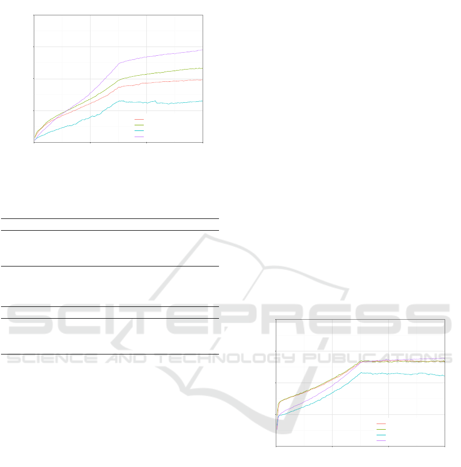
In Figure 3, 4, and 5 the performance score during
training is displayed for the three different state repre-
sentations. In every figure we see the performance of
the agent against the random and semi-deterministic op-
ponent with both the sigmoid and Elu activation func-
tion. For every 10,000 games played we plot the per-
formance score, which ranges from 0 to 1. We see
that for all three state representations performance in-
creases strongly as long as some explorative actions are
made. When exploration stops at 750,000 games, perfor-
mance stays approximately the same, except for the full
grid state representation with the Elu activation function
against the semi-deterministic opponent. We have also
experimented with a constant exploration of 10% and
with exploration gradually falling to 0% over all train-
ing games, however this did not lead to better perfor-
mances. After training the agent, we tested the agent’s
performance on 10,000 test games. The results are dis-
played in Table 1 and 2. These results are gathered from
ten independent trials, for which also the standard error
is reported.
From Table 1 and 2 we can conclude that with the
sigmoid activation function, the use of vision grids in-
creases the performance of the agent when compared to
0.25
0.50
0.75
1.00
0 50 100 150 200 250
Games played
% correct predicted
Small_VG
Large_VG
Full_Grid
Prediction against semi−deterministic opponent
0.25
0.50
0.75
1.00
0 50 100 150 200 250
Games played
% correct predicted
Small_VG
Large_VG
Full_Grid
Prediction against semi−deterministic opponent
0.25
0.50
0.75
1.00
0 50 100 150 200 250
Games played
% correct predicted
Small_VG
Large_VG
Full_Grid
Prediction against semi−deterministic opponent
0.25
0.50
0.75
1.00
0 50 100 150 200 250
Games played
% correct predicted
Small_VG
Large_VG
Full_Grid
Prediction against semi−deterministic opponent
x100
0.25
0.50
0.75
1.00
0 50 100 150 200 250
Games played
% correct predicted
Small_VG
Large_VG
Full_Grid
Prediction against semi−deterministic opponent
x100
0.25
0.50
0.75
1.00
0 50 100 150 200 250
Games played
% correct predicted
Small_VG
Large_VG
Full_Grid
Prediction against semi−deterministic opponent
x100
0.25
0.50
0.75
1.00
0 50 100 150 200 250
Games played
% correct predicted
Small_VG
Large_VG
Full_Grid
Prediction against semi−deterministic opponent
x100
0.25
0.50
0.75
1.00
0 50 100 150 200 250
Games played
% correct predicted
Small_VG
Large_VG
Full_Grid
Prediction against semi−deterministic opponent
x100
0.25
0.50
0.75
1.00
0 50 100 150 200 250
Games played
% correct predicted
Small_VG
Large_VG
Full_Grid
Prediction against semi−deterministic opponent
x100
0.25
0.50
0.75
1.00
0 50 100 150 200 250
Games played
% correct predicted
Small_VG
Large_VG
Full_Grid
Prediction against semi−deterministic opponent
x100
0.25
0.50
0.75
1.00
0 50 100 150 200 250
Games played
% correct predicted
Small_VG
Large_VG
Full_Grid
Prediction against semi−deterministic opponent
x10
4
0.25
0.50
0.75
1.00
0 50 100 150 200 250
Games played
Performance score
Small_VG
Large_VG
Full_Grid
Training performance large vision grids opponent modelling
x10
4
0.25
0.50
0.75
1.00
0 50 100 150 200 250
Games played
Performance score
Random_Sigmoid
Random_Elu
Deterministic_Sigmoid
Deterministic_Elu
Training performance large vision grids opponent modelling
0.25
0.50
0.75
1.00
0 50 100 150
Games played
Performance score
Random_Sigmoid
Random_Elu
Deterministic_Sigmoid
Deterministic_Elu
Training performance large vision grids opponent modelling
0.25
0.50
0.75
1.00
0 50 100 150
Games played
Performance score
Random_Sigmoid
Random_Elu
Deterministic_Sigmoid
Deterministic_Elu
Training performance large vision grids opponent modelling
0.25
0.50
0.75
1.00
0 50 100 150
Games played
Performance score
Random_Sigmoid
Random_Elu
Deterministic_Sigmoid
Deterministic_Elu
Training performance large vision grids opponent modelling
x10
4
0.25
0.50
0.75
1.00
0 50 100 150
Games played
Performance score
Random_Sigmoid
Random_Elu
Deterministic_Sigmoid
Deterministic_Elu
Training performance large vision grids opponent modelling
x10
4
0.25
0.50
0.75
1.00
0 50 100 150
Games played
Performance score
Random_Sigmoid
Random_Elu
Deterministic_Sigmoid
Deterministic_Elu
Training performance large vision grids opponent modelling
x10
4
0.25
0.50
0.75
1.00
0 50 100 150
Games played
Performance score
Random_Sigmoid
Random_Elu
Deterministic_Sigmoid
Deterministic_Elu
Training performance large vision grids opponent modelling
x10
4
0.25
0.50
0.75
1.00
0 50 100 150
Games played
Performance score
Random_Sigmoid
Random_Elu
Deterministic_Sigmoid
Deterministic_Elu
Training performance large vision grids opponent modelling
x10
4
0.25
0.50
0.75
1.00
0 50 100 150
Games played
Performance score
Random_Sigmoid
Random_Elu
Deterministic_Sigmoid
Deterministic_Elu
Training performance large vision grids
x10
4
0.25
0.50
0.75
1.00
0 50 100 150
Games played
Performance score
Random_Sigmoid
Random_Elu
Deterministic_Sigmoid
Deterministic_Elu
Training performance large vision grids opponent modelling
x10
4
0.25
0.50
0.75
1.00
0 50 100 150
Games played
Performance score
Random_Sigmoid
Random_Elu
Deterministic_Sigmoid
Deterministic_Elu
Training performance small vision grids opponent modelling
x10
4
0.25
0.50
0.75
1.00
0 50 100 150
Games played
Performance score
Random_Sigmoid
Random_Elu
Deterministic_Sigmoid
Deterministic_Elu
Training performance small vision grids
Figure 3: Performance score for small vision grids as state
representation over 1.5 million training games. Note that
after 750,000 games the agent stops performing exploration
moves.
0.25
0.50
0.75
1.00
0 50 100 150 200 250
Games played
% correct predicted
Small_VG
Large_VG
Full_Grid
Prediction against semi−deterministic opponent
0.25
0.50
0.75
1.00
0 50 100 150 200 250
Games played
% correct predicted
Small_VG
Large_VG
Full_Grid
Prediction against semi−deterministic opponent
0.25
0.50
0.75
1.00
0 50 100 150 200 250
Games played
% correct predicted
Small_VG
Large_VG
Full_Grid
Prediction against semi−deterministic opponent
0.25
0.50
0.75
1.00
0 50 100 150 200 250
Games played
% correct predicted
Small_VG
Large_VG
Full_Grid
Prediction against semi−deterministic opponent
x100
0.25
0.50
0.75
1.00
0 50 100 150 200 250
Games played
% correct predicted
Small_VG
Large_VG
Full_Grid
Prediction against semi−deterministic opponent
x100
0.25
0.50
0.75
1.00
0 50 100 150 200 250
Games played
% correct predicted
Small_VG
Large_VG
Full_Grid
Prediction against semi−deterministic opponent
x100
0.25
0.50
0.75
1.00
0 50 100 150 200 250
Games played
% correct predicted
Small_VG
Large_VG
Full_Grid
Prediction against semi−deterministic opponent
x100
0.25
0.50
0.75
1.00
0 50 100 150 200 250
Games played
% correct predicted
Small_VG
Large_VG
Full_Grid
Prediction against semi−deterministic opponent
x100
0.25
0.50
0.75
1.00
0 50 100 150 200 250
Games played
% correct predicted
Small_VG
Large_VG
Full_Grid
Prediction against semi−deterministic opponent
x100
0.25
0.50
0.75
1.00
0 50 100 150 200 250
Games played
% correct predicted
Small_VG
Large_VG
Full_Grid
Prediction against semi−deterministic opponent
x100
0.25
0.50
0.75
1.00
0 50 100 150 200 250
Games played
% correct predicted
Small_VG
Large_VG
Full_Grid
Prediction against semi−deterministic opponent
x10
4
0.25
0.50
0.75
1.00
0 50 100 150 200 250
Games played
Performance score
Small_VG
Large_VG
Full_Grid
Training performance large vision grids opponent modelling
x10
4
0.25
0.50
0.75
1.00
0 50 100 150 200 250
Games played
Performance score
Random_Sigmoid
Random_Elu
Deterministic_Sigmoid
Deterministic_Elu
Training performance large vision grids opponent modelling
0.25
0.50
0.75
1.00
0 50 100 150
Games played
Performance score
Random_Sigmoid
Random_Elu
Deterministic_Sigmoid
Deterministic_Elu
Training performance large vision grids opponent modelling
0.25
0.50
0.75
1.00
0 50 100 150
Games played
Performance score
Random_Sigmoid
Random_Elu
Deterministic_Sigmoid
Deterministic_Elu
Training performance large vision grids opponent modelling
0.25
0.50
0.75
1.00
0 50 100 150
Games played
Performance score
Random_Sigmoid
Random_Elu
Deterministic_Sigmoid
Deterministic_Elu
Training performance large vision grids opponent modelling
x10
4
0.25
0.50
0.75
1.00
0 50 100 150
Games played
Performance score
Random_Sigmoid
Random_Elu
Deterministic_Sigmoid
Deterministic_Elu
Training performance large vision grids opponent modelling
x10
4
0.25
0.50
0.75
1.00
0 50 100 150
Games played
Performance score
Random_Sigmoid
Random_Elu
Deterministic_Sigmoid
Deterministic_Elu
Training performance large vision grids opponent modelling
x10
4
0.25
0.50
0.75
1.00
0 50 100 150
Games played
Performance score
Random_Sigmoid
Random_Elu
Deterministic_Sigmoid
Deterministic_Elu
Training performance large vision grids opponent modelling
x10
4
0.25
0.50
0.75
1.00
0 50 100 150
Games played
Performance score
Random_Sigmoid
Random_Elu
Deterministic_Sigmoid
Deterministic_Elu
Training performance large vision grids opponent modelling
x10
4
0.25
0.50
0.75
1.00
0 50 100 150
Games played
Performance score
Random_Sigmoid
Random_Elu
Deterministic_Sigmoid
Deterministic_Elu
Training performance large vision grids
Figure 4: Performance score for large vision grids as state
representation over 1.5 million training games.
using the full grid. Against the random opponent, the
small vision grid with the Elu activation function per-
forms best. Striking is the performance of the agent us-
ing the full grid against the semi-deterministic opponent
using the Elu activation function, which can be found
in Table 2. The agent reaches a performance score of
0.72 in this case, which is the highest performance score
obtained. This finding might be caused by the fact that
the agent can actually profit from the semi-deterministic
policy the opponent is following, which it detects when
the full grid is used as state representation because it
provides more information about the past moves of the
opponent. Against both opponents, the use of the Elu
activation function with the full-grid representation per-
forms significantly better than the sigmoid function.
Opponent Modelling in the Game of Tron using Reinforcement Learning
35

x10
4
0.25
0.50
0.75
1.00
0 50 100 150
Games played
Performance score
Random_Sigmoid
Random_Elu
Deterministic_Sigmoid
Deterministic_Elu
Training performance full grid
Figure 5: Performance score for the full grid as state repre-
sentation over 1.5 million training games.
Table 1: Performance score and standard errors against the
random opponent.
State representation Sigmoid Elu
Small vision grids 0.56 (0.037) 0.62 (0.019)
Large vision grids 0.54 (0.036) 0.53 (0.022)
Full grid 0.49 (0.017) 0.58 (0.025)
Table 2: Performance score and standard errors against the
deterministic opponent.
State representation Sigmoid Elu
Small vision grids 0.35 (0.044) 0.39 (0.016)
Large vision grids 0.37 (0.034) 0.39 (0.025)
Full grid 0.31 (0.023) 0.72 (0.007)
5.2 Opponent Modelling without
Monte-Carlo Roll-outs
Opponent modelling requires information not only about
the agent’s current position, but also about the oppo-
nent’s position. As explained in section 4, this increases
the number of vision grids used and therefore affects the
number of inputs and best found number of hidden nodes
of the MLP. In the basic case where the full grid is used,
the number of input nodes increases to 300 and the num-
ber of hidden nodes stays 300. For the large vision grids
the number of input nodes increases to 175 and the num-
ber of hidden nodes increases to 300. Finally, when us-
ing the small vision grids the number of input nodes be-
comes 63 and the number of hidden nodes increases to
200. In all networks with opponent modelling the num-
ber of output nodes is eight (the 4 Q-values for the dif-
ferent actions and the 4 outputs to model the opponent’s
probability of selecting that action).
For these experiments preliminary experiments
showed that decreasing the exploration from 10% to 0%
over the first 750,000 games led to the best results in
most cases. However, with large vision grids and the sig-
moid activation function against the random opponent,
exploration decreases from 10% to 0% over 1 million
training games. The learning rate α and discount factor
γ are for the opponent modelling experiments also 0.005
and 0.95 respectively. These values have been found to
lead to the best results, however there are some excep-
tions. When the full grid is used as state representation
in combination with the sigmoid activation function, the
learning rate is lowered to 0.001. This lower learning
rate is also used with small vision grids and the sig-
moid activation function against the random opponent.
Finally, when large vision grids are used in combination
with the sigmoid activation function against the random
opponent, a learning rate of 0.0025 is used. Similar to
the previous experiments, all weights and biases of the
neural networks are randomly initialised between −0.5
and 0.5.
For the opponent modelling experiments we trained
the agent against both opponents and with both acti-
vation functions. We note that in this experiment, no
roll-outs are performed. Therefore any possible perfor-
mance improvement is caused by the additional state in-
formation or the use of the additional outputs that learn
to model the opponent. The latter could be helpful to
learn better features in the hidden layer. Figures 6, 7,
and 8 show the training performance for the three dif-
ferent state representations. Table 3 and 4 show the per-
formance during the 10,000 test games after training the
agent with opponent modelling.
0.25
0.50
0.75
1.00
0 50 100 150 200 250
Games played
% correct predicted
Small_VG
Large_VG
Full_Grid
Prediction against semi−deterministic opponent
0.25
0.50
0.75
1.00
0 50 100 150 200 250
Games played
% correct predicted
Small_VG
Large_VG
Full_Grid
Prediction against semi−deterministic opponent
0.25
0.50
0.75
1.00
0 50 100 150 200 250
Games played
% correct predicted
Small_VG
Large_VG
Full_Grid
Prediction against semi−deterministic opponent
0.25
0.50
0.75
1.00
0 50 100 150 200 250
Games played
% correct predicted
Small_VG
Large_VG
Full_Grid
Prediction against semi−deterministic opponent
x100
0.25
0.50
0.75
1.00
0 50 100 150 200 250
Games played
% correct predicted
Small_VG
Large_VG
Full_Grid
Prediction against semi−deterministic opponent
x100
0.25
0.50
0.75
1.00
0 50 100 150 200 250
Games played
% correct predicted
Small_VG
Large_VG
Full_Grid
Prediction against semi−deterministic opponent
x100
0.25
0.50
0.75
1.00
0 50 100 150 200 250
Games played
% correct predicted
Small_VG
Large_VG
Full_Grid
Prediction against semi−deterministic opponent
x100
0.25
0.50
0.75
1.00
0 50 100 150 200 250
Games played
% correct predicted
Small_VG
Large_VG
Full_Grid
Prediction against semi−deterministic opponent
x100
0.25
0.50
0.75
1.00
0 50 100 150 200 250
Games played
% correct predicted
Small_VG
Large_VG
Full_Grid
Prediction against semi−deterministic opponent
x100
0.25
0.50
0.75
1.00
0 50 100 150 200 250
Games played
% correct predicted
Small_VG
Large_VG
Full_Grid
Prediction against semi−deterministic opponent
x100
0.25
0.50
0.75
1.00
0 50 100 150 200 250
Games played
% correct predicted
Small_VG
Large_VG
Full_Grid
Prediction against semi−deterministic opponent
x10
4
0.25
0.50
0.75
1.00
0 50 100 150 200 250
Games played
Performance score
Small_VG
Large_VG
Full_Grid
Training performance large vision grids opponent modelling
x10
4
0.25
0.50
0.75
1.00
0 50 100 150 200 250
Games played
Performance score
Random_Sigmoid
Random_Elu
Deterministic_Sigmoid
Deterministic_Elu
Training performance large vision grids opponent modelling
0.25
0.50
0.75
1.00
0 50 100 150
Games played
Performance score
Random_Sigmoid
Random_Elu
Deterministic_Sigmoid
Deterministic_Elu
Training performance large vision grids opponent modelling
0.25
0.50
0.75
1.00
0 50 100 150
Games played
Performance score
Random_Sigmoid
Random_Elu
Deterministic_Sigmoid
Deterministic_Elu
Training performance large vision grids opponent modelling
0.25
0.50
0.75
1.00
0 50 100 150
Games played
Performance score
Random_Sigmoid
Random_Elu
Deterministic_Sigmoid
Deterministic_Elu
Training performance large vision grids opponent modelling
x10
4
0.25
0.50
0.75
1.00
0 50 100 150
Games played
Performance score
Random_Sigmoid
Random_Elu
Deterministic_Sigmoid
Deterministic_Elu
Training performance large vision grids opponent modelling
x10
4
0.25
0.50
0.75
1.00
0 50 100 150
Games played
Performance score
Random_Sigmoid
Random_Elu
Deterministic_Sigmoid
Deterministic_Elu
Training performance large vision grids opponent modelling
x10
4
0.25
0.50
0.75
1.00
0 50 100 150
Games played
Performance score
Random_Sigmoid
Random_Elu
Deterministic_Sigmoid
Deterministic_Elu
Training performance large vision grids opponent modelling
x10
4
0.25
0.50
0.75
1.00
0 50 100 150
Games played
Performance score
Random_Sigmoid
Random_Elu
Deterministic_Sigmoid
Deterministic_Elu
Training performance large vision grids opponent modelling
x10
4
0.25
0.50
0.75
1.00
0 50 100 150
Games played
Performance score
Random_Sigmoid
Random_Elu
Deterministic_Sigmoid
Deterministic_Elu
Training performance large vision grids
x10
4
0.25
0.50
0.75
1.00
0 50 100 150
Games played
Performance score
Random_Sigmoid
Random_Elu
Deterministic_Sigmoid
Deterministic_Elu
Training performance large vision grids opponent modelling
x10
4
0.25
0.50
0.75
1.00
0 50 100 150
Games played
Performance score
Random_Sigmoid
Random_Elu
Deterministic_Sigmoid
Deterministic_Elu
Training performance small vision grids opponent modelling
Figure 6: Performance score for small vision grids as state
representation over 1.5 million training games with oppo-
nent modelling but without rollouts.
When we compare these results with the results ob-
tained without opponent modelling, we observe several
differences. First of all, when the full grid is used as
state representation the performance drops with oppo-
nent modelling. The opposite holds for both small and
large vision grids, where performance increases with
opponent modelling. The most significant increase in
performance appears with large vision grids against the
semi-deterministic opponent, where a performance score
of 0.90 is obtained.
In order to test whether this increase in performance
with vision grids arises due to the opponent modelling
ICAART 2018 - 10th International Conference on Agents and Artificial Intelligence
36

0.25
0.50
0.75
1.00
0 50 100 150 200 250
Games played
% correct predicted
Small_VG
Large_VG
Full_Grid
Prediction against semi−deterministic opponent
0.25
0.50
0.75
1.00
0 50 100 150 200 250
Games played
% correct predicted
Small_VG
Large_VG
Full_Grid
Prediction against semi−deterministic opponent
0.25
0.50
0.75
1.00
0 50 100 150 200 250
Games played
% correct predicted
Small_VG
Large_VG
Full_Grid
Prediction against semi−deterministic opponent
0.25
0.50
0.75
1.00
0 50 100 150 200 250
Games played
% correct predicted
Small_VG
Large_VG
Full_Grid
Prediction against semi−deterministic opponent
x100
0.25
0.50
0.75
1.00
0 50 100 150 200 250
Games played
% correct predicted
Small_VG
Large_VG
Full_Grid
Prediction against semi−deterministic opponent
x100
0.25
0.50
0.75
1.00
0 50 100 150 200 250
Games played
% correct predicted
Small_VG
Large_VG
Full_Grid
Prediction against semi−deterministic opponent
x100
0.25
0.50
0.75
1.00
0 50 100 150 200 250
Games played
% correct predicted
Small_VG
Large_VG
Full_Grid
Prediction against semi−deterministic opponent
x100
0.25
0.50
0.75
1.00
0 50 100 150 200 250
Games played
% correct predicted
Small_VG
Large_VG
Full_Grid
Prediction against semi−deterministic opponent
x100
0.25
0.50
0.75
1.00
0 50 100 150 200 250
Games played
% correct predicted
Small_VG
Large_VG
Full_Grid
Prediction against semi−deterministic opponent
x100
0.25
0.50
0.75
1.00
0 50 100 150 200 250
Games played
% correct predicted
Small_VG
Large_VG
Full_Grid
Prediction against semi−deterministic opponent
x100
0.25
0.50
0.75
1.00
0 50 100 150 200 250
Games played
% correct predicted
Small_VG
Large_VG
Full_Grid
Prediction against semi−deterministic opponent
x10
4
0.25
0.50
0.75
1.00
0 50 100 150 200 250
Games played
Performance score
Small_VG
Large_VG
Full_Grid
Training performance large vision grids opponent modelling
x10
4
0.25
0.50
0.75
1.00
0 50 100 150 200 250
Games played
Performance score
Random_Sigmoid
Random_Elu
Deterministic_Sigmoid
Deterministic_Elu
Training performance large vision grids opponent modelling
0.25
0.50
0.75
1.00
0 50 100 150
Games played
Performance score
Random_Sigmoid
Random_Elu
Deterministic_Sigmoid
Deterministic_Elu
Training performance large vision grids opponent modelling
0.25
0.50
0.75
1.00
0 50 100 150
Games played
Performance score
Random_Sigmoid
Random_Elu
Deterministic_Sigmoid
Deterministic_Elu
Training performance large vision grids opponent modelling
0.25
0.50
0.75
1.00
0 50 100 150
Games played
Performance score
Random_Sigmoid
Random_Elu
Deterministic_Sigmoid
Deterministic_Elu
Training performance large vision grids opponent modelling
x10
4
0.25
0.50
0.75
1.00
0 50 100 150
Games played
Performance score
Random_Sigmoid
Random_Elu
Deterministic_Sigmoid
Deterministic_Elu
Training performance large vision grids opponent modelling
x10
4
0.25
0.50
0.75
1.00
0 50 100 150
Games played
Performance score
Random_Sigmoid
Random_Elu
Deterministic_Sigmoid
Deterministic_Elu
Training performance large vision grids opponent modelling
x10
4
0.25
0.50
0.75
1.00
0 50 100 150
Games played
Performance score
Random_Sigmoid
Random_Elu
Deterministic_Sigmoid
Deterministic_Elu
Training performance large vision grids opponent modelling
x10
4
0.25
0.50
0.75
1.00
0 50 100 150
Games played
Performance score
Random_Sigmoid
Random_Elu
Deterministic_Sigmoid
Deterministic_Elu
Training performance large vision grids opponent modelling
x10
4
0.25
0.50
0.75
1.00
0 50 100 150
Games played
Performance score
Random_Sigmoid
Random_Elu
Deterministic_Sigmoid
Deterministic_Elu
Training performance large vision grids
x10
4
0.25
0.50
0.75
1.00
0 50 100 150
Games played
Performance score
Random_Sigmoid
Random_Elu
Deterministic_Sigmoid
Deterministic_Elu
Training performance large vision grids opponent modelling
Figure 7: Performance score for large vision grids as state
representation over 1.5 million training games with oppo-
nent modelling but without rollouts.
0.25
0.50
0.75
1.00
0 50 100 150 200 250
Games played
% correct predicted
Small_VG
Large_VG
Full_Grid
Prediction against semi−deterministic opponent
0.25
0.50
0.75
1.00
0 50 100 150 200 250
Games played
% correct predicted
Small_VG
Large_VG
Full_Grid
Prediction against semi−deterministic opponent
0.25
0.50
0.75
1.00
0 50 100 150 200 250
Games played
% correct predicted
Small_VG
Large_VG
Full_Grid
Prediction against semi−deterministic opponent
0.25
0.50
0.75
1.00
0 50 100 150 200 250
Games played
% correct predicted
Small_VG
Large_VG
Full_Grid
Prediction against semi−deterministic opponent
x100
0.25
0.50
0.75
1.00
0 50 100 150 200 250
Games played
% correct predicted
Small_VG
Large_VG
Full_Grid
Prediction against semi−deterministic opponent
x100
0.25
0.50
0.75
1.00
0 50 100 150 200 250
Games played
% correct predicted
Small_VG
Large_VG
Full_Grid
Prediction against semi−deterministic opponent
x100
0.25
0.50
0.75
1.00
0 50 100 150 200 250
Games played
% correct predicted
Small_VG
Large_VG
Full_Grid
Prediction against semi−deterministic opponent
x100
0.25
0.50
0.75
1.00
0 50 100 150 200 250
Games played
% correct predicted
Small_VG
Large_VG
Full_Grid
Prediction against semi−deterministic opponent
x100
0.25
0.50
0.75
1.00
0 50 100 150 200 250
Games played
% correct predicted
Small_VG
Large_VG
Full_Grid
Prediction against semi−deterministic opponent
x100
0.25
0.50
0.75
1.00
0 50 100 150 200 250
Games played
% correct predicted
Small_VG
Large_VG
Full_Grid
Prediction against semi−deterministic opponent
x100
0.25
0.50
0.75
1.00
0 50 100 150 200 250
Games played
% correct predicted
Small_VG
Large_VG
Full_Grid
Prediction against semi−deterministic opponent
x10
4
0.25
0.50
0.75
1.00
0 50 100 150 200 250
Games played
Performance score
Small_VG
Large_VG
Full_Grid
Training performance large vision grids opponent modelling
x10
4
0.25
0.50
0.75
1.00
0 50 100 150 200 250
Games played
Performance score
Random_Sigmoid
Random_Elu
Deterministic_Sigmoid
Deterministic_Elu
Training performance large vision grids opponent modelling
0.25
0.50
0.75
1.00
0 50 100 150
Games played
Performance score
Random_Sigmoid
Random_Elu
Deterministic_Sigmoid
Deterministic_Elu
Training performance large vision grids opponent modelling
0.25
0.50
0.75
1.00
0 50 100 150
Games played
Performance score
Random_Sigmoid
Random_Elu
Deterministic_Sigmoid
Deterministic_Elu
Training performance large vision grids opponent modelling
0.25
0.50
0.75
1.00
0 50 100 150
Games played
Performance score
Random_Sigmoid
Random_Elu
Deterministic_Sigmoid
Deterministic_Elu
Training performance large vision grids opponent modelling
x10
4
0.25
0.50
0.75
1.00
0 50 100 150
Games played
Performance score
Random_Sigmoid
Random_Elu
Deterministic_Sigmoid
Deterministic_Elu
Training performance large vision grids opponent modelling
x10
4
0.25
0.50
0.75
1.00
0 50 100 150
Games played
Performance score
Random_Sigmoid
Random_Elu
Deterministic_Sigmoid
Deterministic_Elu
Training performance large vision grids opponent modelling
x10
4
0.25
0.50
0.75
1.00
0 50 100 150
Games played
Performance score
Random_Sigmoid
Random_Elu
Deterministic_Sigmoid
Deterministic_Elu
Training performance large vision grids opponent modelling
x10
4
0.25
0.50
0.75
1.00
0 50 100 150
Games played
Performance score
Random_Sigmoid
Random_Elu
Deterministic_Sigmoid
Deterministic_Elu
Training performance large vision grids opponent modelling
x10
4
0.25
0.50
0.75
1.00
0 50 100 150
Games played
Performance score
Random_Sigmoid
Random_Elu
Deterministic_Sigmoid
Deterministic_Elu
Training performance large vision grids
x10
4
0.25
0.50
0.75
1.00
0 50 100 150
Games played
Performance score
Random_Sigmoid
Random_Elu
Deterministic_Sigmoid
Deterministic_Elu
Training performance large vision grids opponent modelling
x10
4
0.25
0.50
0.75
1.00
0 50 100 150
Games played
Performance score
Random_Sigmoid
Random_Elu
Deterministic_Sigmoid
Deterministic_Elu
Training performance small vision grids opponent modelling
x10
4
0.25
0.50
0.75
1.00
0 50 100 150
Games played
Performance score
Random_Sigmoid
Random_Elu
Deterministic_Sigmoid
Deterministic_Elu
Training performance small vision grids
x10
4
0.25
0.50
0.75
1.00
0 50 100 150
Games played
Performance score
Random_Sigmoid
Random_Elu
Deterministic_Sigmoid
Deterministic_Elu
Training performance full grid opponent modelling
Figure 8: Performance score for the full grid as state rep-
resentation over 1.5 million training games with opponent
modelling but without rollouts.
Table 3: Performance score and standard errors with oppo-
nent modelling without rollouts against the random oppo-
nent.
State representation Sigmoid Elu
Small vision grids 0.67 (0.004) 0.67 (0.009)
Large vision grids 0.72 (0.005) 0.79 (0.003)
Full grid 0.42 (0.016) 0.40 (0.025)
Table 4: Performance score and standard errors with op-
ponent modelling without rollouts against the deterministic
opponent.
State representation Sigmoid Elu
Small vision grids 0.57 (0.015) 0.69 (0.005)
Large vision grids 0.63 (0.019) 0.90 (0.003)
Full grid 0.32 (0.023) 0.62 (0.015)
technique, we conducted another experiment. In this ex-
periment the set-up is exactly the same as in the oppo-
nent modelling experiment, but now the agent does not
learn to model the opponent. The average results of ten
x100
0.25
0.50
0.75
1.00
0 50 100 150 200 250
Games played
% correct predicted
Small_VG
Large_VG
Full_Grid
Prediction against random opponent
Figure 9: Percentage of moves correctly predicted against
the random opponent.
test games with the Elu activation function can be found
in Table 5.
Table 5: Performance score and standard errors with the Elu
activation function and opponent vision grids, but without
opponent modelling.
State representation Random Deterministic
Small vision grids 0.69 (0.008) 0.69 (0.003)
Large vision grids 0.82 (0.009) 0.89 (0.003)
From Table 5 we can conclude that the agent’s in-
crease in performance with opponent modelling is due
to the extra vision grids generated. This is the case since
there is not much difference in performance with and
without opponent modelling when the extra vision grids
for opponent modelling are also fed into the MLP.
5.3 Opponent Modelling with
Monte-Carlo Roll-outs
After the agent is trained using opponent modelling, we
applied roll-outs in order to try to increase the perfor-
mance of the agent even further. The number of actions
in a roll-out is set to ten, as this gives the agent the op-
portunity to look far enough in the future to choose the
optimal action. Further increasing the number of actions
of a roll-out will often not benefit the agent, as the aver-
age amount of actions in a game is twenty. We compare
the performance of the agent with one and ten roll-outs.
Since the opponent’s actions within the roll-outs are de-
termined by the learned probability distribution, we plot
the prediction accuracy of the agent against both agents
in Figure 9 and 10. These results are for the Elu acti-
vation function, which learns slightly faster than the sig-
moid activation function. We observe that within 25,000
games the agent correctly predicts 50% of the random
opponent’s moves and 90% of the semi-deterministic op-
ponent’s moves when we use vision grids. When the full
grid is used, this accuracy is equal to 40% and 80% re-
spectively.
Opponent Modelling in the Game of Tron using Reinforcement Learning
37

0.25
0.50
0.75
1.00
0 50 100 150 200 250
Games played
% correct predicted
Small_VG
Large_VG
Full_Grid
Prediction against semi−deterministic opponent
0.25
0.50
0.75
1.00
0 50 100 150 200 250
Games played
% correct predicted
Small_VG
Large_VG
Full_Grid
Prediction against semi−deterministic opponent
0.25
0.50
0.75
1.00
0 50 100 150 200 250
Games played
% correct predicted
Small_VG
Large_VG
Full_Grid
Prediction against semi−deterministic opponent
0.25
0.50
0.75
1.00
0 50 100 150 200 250
Games played
% correct predicted
Small_VG
Large_VG
Full_Grid
Prediction against semi−deterministic opponent
x100
0.25
0.50
0.75
1.00
0 50 100 150 200 250
Games played
% correct predicted
Small_VG
Large_VG
Full_Grid
Prediction against semi−deterministic opponent
x100
0.25
0.50
0.75
1.00
0 50 100 150 200 250
Games played
% correct predicted
Small_VG
Large_VG
Full_Grid
Prediction against semi−deterministic opponent
x100
0.25
0.50
0.75
1.00
0 50 100 150 200 250
Games played
% correct predicted
Small_VG
Large_VG
Full_Grid
Prediction against semi−deterministic opponent
x100
0.25
0.50
0.75
1.00
0 50 100 150 200 250
Games played
% correct predicted
Small_VG
Large_VG
Full_Grid
Prediction against semi−deterministic opponent
x100
0.25
0.50
0.75
1.00
0 50 100 150 200 250
Games played
% correct predicted
Small_VG
Large_VG
Full_Grid
Prediction against semi−deterministic opponent
x100
0.25
0.50
0.75
1.00
0 50 100 150 200 250
Games played
% correct predicted
Small_VG
Large_VG
Full_Grid
Prediction against semi−deterministic opponent
Figure 10: Percentage of moves correctly predicted against
the semi-deterministic opponent.
Table 6: Performance score and standard errors with one
roll-out and a depth of ten actions against the random oppo-
nent.
State representation Sigmoid Elu
Small vision grids 0.83 (0.002) 0.84 (0.003)
Large vision grids 0.66 (0.008) 0.66 (0.004)
Full grid 0.65 (0.004) 0.72 (0.007)
The performance score and standard error using one
roll-out with a horizon of ten steps during 10,000 test
games can be found in Table 6 and 7. The Monte-
Carlo roll-outs further increase the agent’s performance
in most cases. However, performance decreases when
large vision grids are used against the random opponent.
In all other cases, performance considerably increases
with the use of roll-outs. The highest performance score
obtained is 0.98, which is obtained with large vision
grids and the Elu activation function against the semi-
deterministic opponent. This shows that by applying
opponent modelling and Monte-Carlo roll-outs, perfor-
mance can be increased to very high levels. From Ta-
ble 7 we observe that also with small vision grids, per-
formance scores of over 0.90 are obtained against the
semi-deterministic opponent. If we compare the results
with vision grids and the full grid as state representa-
tion, we observe that vision grids significantly increase
performance with opponent modelling and Monte-Carlo
roll-outs. This increase is most evident against the semi-
deterministic opponent. When the opponent employs
the collision-avoiding random policy, small vision grids
lead to the highest performance. When comparing Ta-
ble 3 and 6, we see that roll-outs also increase perfor-
Table 7: Performance score and standard errors with one
roll-out and a depth of ten actions against the deterministic
opponent.
State representation Sigmoid Elu
Small vision grids 0.93 (0.002) 0.96 (0.001)
Large vision grids 0.95 (0.002) 0.98 (0.001)
Full grid 0.54 (0.010) 0.75 (0.010)
Table 8: Performance score and standard errors with ten
roll-outs and a depth of ten actions against the random op-
ponent.
State representation Sigmoid Elu
Small vision grids 0.84 (0.016) 0.88 (0.001)
Large vision grids 0.90 (0.001) 0.91 (0.001)
Full grid 0.72 (0.008) 0.74 (0.009)
Table 9: Performance score and standard errors with ten
roll-outs and a depth of ten actions against the deterministic
opponent.
State representation Sigmoid Elu
Small vision grids 0.93 (0.002) 0.96 (0.001)
Large vision grids 0.96 (0.002) 0.98 (0.001)
Full grid 0.55 (0.008) 0.78 (0.010)
mance against this random opponent. This shows that
although the policy of the opponent is far from deter-
ministic, opponent modelling still significantly increases
performance from 0.67 to 0.83 with the sigmoid activa-
tion function and from 0.67 to 0.84 with the Elu activa-
tion function when small vision grids are used as state
representation.
After applying one roll-out for each action at any
state, we also tested whether increasing the number of
roll-outs to ten would affect the agent’s performance.
The results are displayed in Table 8 and 9. When com-
paring the agent’s performance with one and ten roll-
outs, we detect one noteworthy difference. The agent’s
performance against the random opponent considerably
increases when we use ten instead of one roll-out. This
increase is especially large when we use large vision
grids. Against the semi-deterministic opponent, increas-
ing the number of roll-outs has no noticeable effect. This
is because the agent predicts the semi-deterministic op-
ponent correctly in over 90% of the cases, causing the
advantage of action sampling and multiple roll-outs to
be absent.
In order to determine whether it is the model of the
opponent that allows the agent to attain very high per-
formance levels using roll-outs, we also investigated the
performance of the agent when the moves of the op-
ponent in the roll-outs are determined randomly rather
than from the learned model of the opponent. The re-
sults can be found in Table 10 and 11. From the results,
we can conclude that it is indeed the model of the op-
ponent that increases the agent’s performance when roll-
outs are used, because a bad opponent model results in
much worse performances in combination with roll-outs.
6 CONCLUSION
This paper has shown that vision grids can be used to
overcome the problems associated with applying rein-
forcement learning in problems with large state spaces.
ICAART 2018 - 10th International Conference on Agents and Artificial Intelligence
38

Table 10: Performance score and standard errors with one
roll-outs and a depth of ten actions against the random op-
ponent and without using the learned model of the oppo-
nent.
State representation Sigmoid Elu
Small vision grids 0.46 (0.007) 0.50 (0.001)
Large vision grids 0.50 (0.001) 0.51 (0.002)
Full grid 0.37 (0.010) 0.35 (0.006)
Table 11: Performance score and standard errors with one
roll-outs and a depth of ten actions against the deterministic
opponent and without using the learned model of the oppo-
nent.
State representation Sigmoid Elu
Small vision grids 0.34 (0.003) 0.35 (0.001)
Large vision grids 0.35 (0.001) 0.36 (0.001)
Full grid 0.21 (0.007) 0.21 (0.005)
Using vision grids as state representation not only in-
creased the learning speed, it also increased the agent’s
performance in most cases. From all state represen-
tations, the large vision grids obtain the best perfor-
mances. They reduce the number of different possible
inputs compared to full grids, but contain more informa-
tion that the small vision grids.
This paper also confirms the benefits of the Elu ac-
tivation function over the sigmoid activation function.
Against the semi-deterministic opponent, the Elu ac-
tivation function increased the agent’s performance in
eleven of the twelve conducted experiments and against
the random opponent performance increased in eight of
the twelve experiments. From this it seems that the Elu
activation function performs especially much better than
the sigmoid function in case of less noisy updates due to
the more deterministic opponent.
Finally, the introduced opponent modelling tech-
nique allows the agent to concurrently learn and model
the opponent and in combination with planning algo-
rithms, such as Monte-Carlo roll-outs, it can be used
to significantly increase performance against two widely
different opponents.
An interesting possibility for future research is to test
whether the use of vision grids causes the agent to form
a better generalised policy. We believe that this is the
case, since vision grids are less dependent on the dimen-
sions of the environment and possible obstacles the agent
might encounter. Therefore, the learned policy will bet-
ter generalise to other environments. Finally, the pro-
posed opponent modelling technique is widely applica-
ble and we are interested to see whether it also proves
useful in other problems.
REFERENCES
Bellman, R. (1957). A markovian decision process. Indiana
Univ. Math. J., 6 No. 4:679–684.
Bom, L., Henken, R., and Wiering, M. (2013). Reinforce-
ment learning to train Ms. Pac-Man using higher-order
action-relative inputs. In 2013 IEEE Symposium on
Adaptive Dynamic Programming and Reinforcement
Learning (ADPRL), pages 156–163.
Bouzy, B. and Helmstetter, B. (2004). Monte-Carlo Go
Developments, pages 159–174. Springer US, Boston,
MA.
Clevert, D., Unterthiner, T., and Hochreiter, S. (2015). Fast
and accurate deep network learning by exponential
linear units (elus). CoRR, abs/1511.07289.
Collins, B. (2007). Combining opponent modeling and
model-based reinforcement learning in a two-player
competitive game. Master’s thesis, School of Infor-
matics, University of Edinburgh.
Ganzfried, S. and Sandholm, T. (2011). Game theory-based
opponent modeling in large imperfect-information
games. In the 10th International Conference on
Autonomous Agents and Multiagent Systems-Volume
2, pages 533–540. International Foundation for Au-
tonomous Agents and Multiagent Systems.
He, H., Boyd-Graber, J. L., Kwok, K., and III, H. D. (2016).
Opponent modeling in deep reinforcement learning.
CoRR, abs/1609.05559.
Mealing, R. A. (2015). Dynamic opponent modelling in
two-player games. PhD thesis, University of Manch-
ester, UK.
Mnih, V., Kavukcuoglu, K., Silver, D., Graves, A.,
Antonoglou, I., Wierstra, D., and Riedmiller, M.
(2013). Playing atari with deep reinforcement learn-
ing. arXiv preprint arXiv:1312.5602.
Rumelhart, D. E., Hinton, G. E., and Williams, R. J. (1988).
Neurocomputing: Foundations of Research, chapter
Learning Internal Representations by Error Propaga-
tion, pages 673–695. MIT Press, Cambridge, MA,
USA.
Shantia, A., Begue, E., and Wiering, M. (2011). Con-
nectionist reinforcement learning for intelligent unit
micro management in Starcraft. In Neural Networks
(IJCNN), The 2011 International Joint Conference on,
pages 1794–1801. IEEE.
Sheppard, B. (2002). World-championship-caliber scrab-
ble. Artificial Intelligence, 134(12):241 – 275.
Silver, D., Huang, A., Maddison, C. J., Guez, A., Sifre, L.,
van den Driessche, G., Schrittwieser, J., Antonoglou,
I., Panneershelvam, V., Lanctot, M., Dieleman, S.,
Grewe, D., Nham, J., Kalchbrenner, N., Sutskever, I.,
Lillicrap, T., Leach, M., Kavukcuoglu, K., Graepel,
T., and Hassabis, D. (2016a). Mastering the game of
Go with deep neural networks and tree search. Nature,
529(7587):484–489.
Silver, D., van Hasselt, H., Hessel, M., Schaul, T., Guez,
A., Harley, T., Dulac-Arnold, G., Reichert, D., Rabi-
nowitz, N., Barreto, A., and Degris, T. (2016b). The
predictron: End-to-end learning and planning. CoRR,
abs/1612.08810.
Southey, F., Bowling, M., Larson, B., Piccione, C., Burch,
N., Billings, D., and Rayner, C. (2005). Bayes bluff:
Opponent modelling in poker. In Proceedings of the
Opponent Modelling in the Game of Tron using Reinforcement Learning
39

21st Annual Conference on Uncertainty in Artificial
Intelligence (UAI, pages 550–558.
Sutton, R. S. (1988). Learning to predict by the methods of
temporal differences. Machine Learning, 3(1):9–44.
Sutton, R. S. and Barto, A. G. (1998). Introduction to Re-
inforcement Learning. MIT Press, Cambridge, MA,
USA, 1st edition.
Tesauro, G. (1995). Temporal difference learning and TD-
gammon. Commun. ACM, 38(3):58–68.
Tesauro, G. and Galperin, G. R. (1997). On-line Policy
Improvement using Monte-Carlo Search, pages 1068–
1074. MIT Press.
van Otterlo, M. and Wiering, M. (2012). Reinforcement
Learning and Markov Decision Processes, pages 3–
42. Springer Berlin Heidelberg, Berlin, Heidelberg.
Watkins, C. J. and Dayan, P. (1992). Q-learning. Machine
learning, 8(3):279–292.
ICAART 2018 - 10th International Conference on Agents and Artificial Intelligence
40