Fast 3D Scene Alignment with Stereo Images

using a Stixel-based 3D Model

Dennis W. J. M. van de Wouw

1,2

, Willem P. Sanberg

, Gijs Dubbelman

and Peter H. N. de With

Department of Electrical Engineering, Eindhoven University of Technology, Eindhoven, The Netherlands

ViNotion B.V., Eindhoven, The Netherlands

Keywords:

Image Registration, Real-time, View Synthesis, Stixel-World.

Abstract:

Scene alignment for images recorded from different viewpoints is a challenging task, especially considering

strong parallax effects. This work proposes a diorama-box model for a 2.5D hierarchical alignment approach,

which is speciﬁcally designed for image registration from a moving vehicle using a stereo camera. For this

purpose, the Stixel World algorithm is used to partition the scene into super-pixels, which are transformed

to 3D. This model is further reﬁned by assigning a slanting orientation to each stixel and by interpolating

between stixels, to prevent gaps in the 3D model. The resulting alignment shows promising results, where

under normal viewing conditions, more than 96% of all annotated points are registered with an alignment

error up to 5 pixels at a resolution of 1920 × 1440 pixels, executing at near-real time performance (4 fps) for

the intended application.

1 INTRODUCTION

Image registration is the process of placing two ima-

ges captured from different viewpoints in the same

coordinate system. It ensures that pixels represen-

ting the same world point in both images, map to the

same image coordinates after successful registration.

This is relevant in many applications, such as medical

image analysis, object recognition, image stitching

and change detection (van de Wouw et al., 2016). Es-

pecially for the latter application, an accurate align-

ment is crucial as it enables pixel-wise comparisons

between the two images.

Image registration becomes quite challenging

when considering images acquired from a moving

vehicle in an urban environment, which is the focus

of this work. In a repetitive capturing scenario, ima-

ges are typically acquired from different viewpoints,

while signiﬁcant time may have passed between cap-

turing the historic image and the live image. This po-

ses additional challenges, where the registration now

has to cope with dynamic appearance changes of the

scene, as well as strong parallax effects.

Appearance changes are generally unavoidable

when recording outdoors at different moments in

time. Changes in lighting and different weather con-

ditions may signiﬁcantly affect the colors and con-

trast of a scene. Furthermore, there may be dynamic

changes in the scene, such as other trafﬁc participants

and objects placed in or removed from the scene in

between the recordings moments. Although such an

object may only exist in either the historic image or

the live image, it should still be aligned to the cor-

rect part of the other image. As a result, regular ﬂow-

based methods cannot be used to align such objects as

they are not present in both images (Werlberger et al.,

2010).

Another challenge is parallax, which results in a

difference between the apparent positions of an object

viewed along two different lines of sight, e.g. when

images are captured from different viewpoints. As

a consequence, the relative position and even the or-

dering of objects in the historic and live image may

change when capturing the same scene from two dif-

ferent viewpoints. This is depicted in Figure 1, where

the object ordering changes from A-B-C-D to A-C-

B-D. This change in relative positions of the objects,

depending on their 3D position in the scene, can no

longer be handled by a global-afﬁne transformation

of the images.

To overcome the parallax issue, the registration

problem can be solved in 3D, where the positioning

of objects is uniquely deﬁned. By aligning the 3D

point clouds and projecting the results back to 2D,

parallax is handled correctly. However, since our 3D

points are estimated from a stereo camera using dis-

250

Wouw, D., Sanberg, W., Dubbelman, G. and With, P.

Fast 3D Scene Alignment with Stereo Images using a Stixel-based 3D Model.

DOI: 10.5220/0006535302500259

In Proceedings of the 13th International Joint Conference on Computer Vision, Imaging and Computer Graphics Theory and Applications (VISIGRAPP 2018) - Volume 4: VISAPP, pages

250-259

ISBN: 978-989-758-290-5

Figure 1: Sample images showing the same scene from dif-

ferent viewpoints. Note the perspective distortion and the

parallax effect, i.e. the same lighting pole C is located in

front of A in the left image, while it is in front of B in the

right image.

parity estimation, they are not sufﬁciently accurate for

a direct projection. Instead, a model-based projection

is required that is robust against noise in the 3D-point

cloud. For this purpose and as an initial step, we adopt

the hierarchical 2.5D alignment approach introduced

in (van de Wouw et al., 2016), which is explained

in Section 3. This adopted approach is only able to

align the non-linear ground surface, but not the ob-

jects above the ground surface. Therefore and as a

next step, the main focus of this work is to extend the

alignment to the entire scene, including 3D objects.

The remainder of this paper is organized as fol-

lows. In the next section, the proposed method is laid

out to related work on image registration under view-

point differences and 3D scene modeling. Section 3

summarizes the baseline image registration method.

Section 4 details the proposed method, followed by a

validation of our method in Section 5. A discussion

on the application of the proposed work is given in

Section 6. Finally, Section 7 presents conclusions.

2 RELATED WORK

2.1 Image Registration under

Viewpoint Differences

To handle perspective distortion during alignment of

images from different viewpoints, several approaches

exist. The ﬁrst approach involves segmenting the 2D

scene into sufﬁciently small parts, such that for each

part an individual afﬁne transformation exists to re-

gister it to the target image or to a common coordi-

nate system. For this purpose, the authors of (Zhang

et al., 2016) and (Su and Lai, 2015) use a mesh-based

approach, where they divide the image into a grid

and for each cell ﬁnd a local afﬁne transformation.

This way, they can accommodate moderate deviati-

ons from planar structures. Lou and Gevers (Lou and

Gevers, 2014) ﬁrst segment the scene into planar regi-

ons and ﬁnd an afﬁne transformation for every plane,

in theory allowing to prevent the parallax issues il-

lustrated in Figure 1. Although these methods show

promising results, they cannot be performed in real-

time, making them less suited to be used while dri-

ving, which is the aim of our work.

Another approach is to solve the alignment in 3D.

As a change in viewpoint does not alter the relative 3D

positions of the objects in the scene, the problem sim-

pliﬁes to estimating a rigid transformation. The alig-

ned 3D point cloud is then projected back to 2D, such

that the historic scene is rendered from the live camera

viewpoint. The naive approach would transform each

individual point in the point cloud and project it to

2D separately. However, this causes signiﬁcant holes

in the resulting image, which become more apparent

when viewpoint differences are considered. Alterna-

tively, a hierarchical 2.5D alignment (van de Wouw

et al., 2016) can be employed. This method applies a

rigid 3D transformation to a textured polygon model

of the historic scene, after which the transformed mo-

del is projected back to 2D. This results in a registe-

red image without holes in which parallax is handled

correctly, i.e. the objects are in the correct positions

in the 2D image. Moreover, this strategy allows for

real-time execution while driving. For this reason, we

build further upon this method in our current work.

2.2 3D Scene Modeling

Projecting textured surfaces outperforms per-pixel

processing, since it facilitates addressing holes and

noise in the depth data. For this purpose, we require a

3D surface model for the full scene. In the ﬁeld of 3D

reconstruction, meshes are a common data represen-

tation. These meshes are often acquired via a Delau-

nay triangulation of measured point clouds. Typically,

these algorithms aim at single object reconstruction

(such as digitizing statues and the like, for cultural

preservation), but several methods are also employed

in our context: outdoor scene modeling. These sys-

tems achieve a high level of geometric accuracy in the

data that is captured close to the objects in the scene,

e.g. facade modeling with accurate ridges and win-

dow stills, etc. (Salman and Yvinec, 2010) (Chauve

et al., 2010), or detailed rock-mass-surface and stai-

rcases (Maiti and Chakravarty, 2016). However, the

processing times of these algorithms lies in the or-

der of seconds (Salman and Yvinec, 2010) (Maiti and

Chakravarty, 2016) or even minutes (Labatut et al.,

2009) (Chauve et al., 2010) per scene, which does

not satisfy our real-time processing constraints. Mo-

reover, our system does not need that level of detail.

Faster pipelines exist, but typically provide 3D mo-

dels that are too sparse or coarse (Natour et al., 2015),

Fast 3D Scene Alignment with Stereo Images using a Stixel-based 3D Model

251

whereas we need dense modeling.

Alternative modeling strategies can be derived

from algorithms that are predominantly designed for

image segmentation instead of 3D modeling, namely:

super-pixel methods. In general, they have been de-

signed to process 2D color images, such as LV (Fel-

zenszwalb and Huttenlocher, 2004), SLIC (Achanta

et al., 2012) and SEOF (Veksler et al., 2010). Each

of these has its own various extensions to incorporate

2.5D or point cloud data. Extensions for LV involve

LVPCS (Strom et al., 2010), MLVS (Sanberg et al.,

2013) and GBIS+D (Cordts et al., 2016), SLIC is ex-

tended in StereoSLIC (Yamaguchi et al., 2014), and

SEOF is modiﬁed into SEOF+D (Cordts et al., 2016).

Although all of these methods can provide relevant

super-pixel segmentations, the resulting super-pixels

are shaped irregularly, yielding an inefﬁcient repre-

sentation. Moreover, they need to be calculated on

the whole image at once. For trading off modeling

ﬂexibility versus optimality and computational com-

plexity, the Stixel World has been introduced (Pfeif-

fer, 2012). This probabilistic super-pixel method has

been designed speciﬁcally for the context of intelli-

gent vehicles, aiming at providing a compact yet ro-

bust representation of trafﬁc scenes in front of a vehi-

cle, which can be generated efﬁciently in real time.

The Stixel World algorithm relies on disparity data

to partition scenes into vertically stacked, rectangu-

lar patches of a certain height and 3D position with

respect to the camera sensor. These rectangular pat-

ches are labeled as either ground or obstacle during

the segmentation process, thereby providing a seman-

tic segmentation as well as a 3D representation. Mo-

reover, stixels can be computed efﬁciently using Dyn-

amic Programming, where multiple columns of dispa-

rity measurements are processed in parallel (Pfeiffer,

2012).

Another specialized scene modeling method for

intelligent vehicles relies on 3D voxels (Broggi et al.,

2013). It generates and removes cubic voxels to

handle the dynamic aspect of a trafﬁc scene and stores

them efﬁciently in an octree-based fashion. However,

it relies on tracking the voxels over time and does not

employ any real-world regularization. Since our sy-

stem operates at a low frame rate (±6 fps), but at a

much higher resolution (above HD instead of VGA),

this method is likely to provide noisy and spurious

false detections.

Considering the methods described above, we

propose to avoid modeling of the entire scene into an

expensive detailed mesh, or in a voxel grid without

strict regularization. Instead, we introduce a simpli-

ﬁed 3D model, which we refer to as the ’diorama-box

model’, shown in Figure 3. This model extends the

non-linear surface model from (van de Wouw et al.,

2016) with 3D objects, where objects are modeled by

one or more slanted planar regions (in 3D) estima-

ted from a Stixel World representation. The proposed

model allows for real-time computation.

The main contributions of this paper are as fol-

lows. First, we introduce an efﬁcient 3D scene mo-

del to be used in the 2.5D hierarchical alignment

approach (van de Wouw et al., 2016), by including

super-pixels obtained through the Stixel World algo-

rithm into the existing ground model. Second, we

improve the consistency of the 3D model by adap-

ting the obtained stixel-based model. Finally, we

validate the proposed model by employing it in our

scene-alignment approach and generally show that the

registration error is below 5 pixels for HD+ images

(1920 × 1440 pixels).

3 BASELINE IMAGE

REGISTRATION

The 2.5D hierarchical alignment approach (van de

Wouw et al., 2016) aims at aligning two images of

the same scene that are captured from different view-

points. It builds on the idea that registration errors due

to parallax can be avoided when aligning the 3D point

clouds, instead of directly transforming the 2D ima-

ges. For this purpose, a 3D scene model of the historic

scene is constructed onto which the historic texture is

projected. Next, this textured model is transformed to

the coordinate system of the live image. The transfor-

med model is then projected back to 2D, which ren-

ders the historic image as if seen by the live camera.

Finally, small misalignments after initial registration

are corrected by a registration reﬁnement based on op-

tical ﬂow. This approach is summarized in Figure 2.

The 3D transformation (pose) estimation from Fi-

gure 2 lies outside the scope of this paper and is des-

cribed in more detail in (van de Wouw et al., 2017).

The current work focuses on the 3D scene recon-

struction and aims at registering the historic image to

the live image in 2D.

It should be noted that we are not necessarily in-

terested in 3D model accuracy, as long as the model

is able to simulate the 2D aligned image with a low

registration error. In a similar fashion, the pose esti-

mation also minimizes the registration error after pro-

jection to 2D, instead of establishing the 3D pose in

world coordinates.

VISAPP 2018 - International Conference on Computer Vision Theory and Applications

252

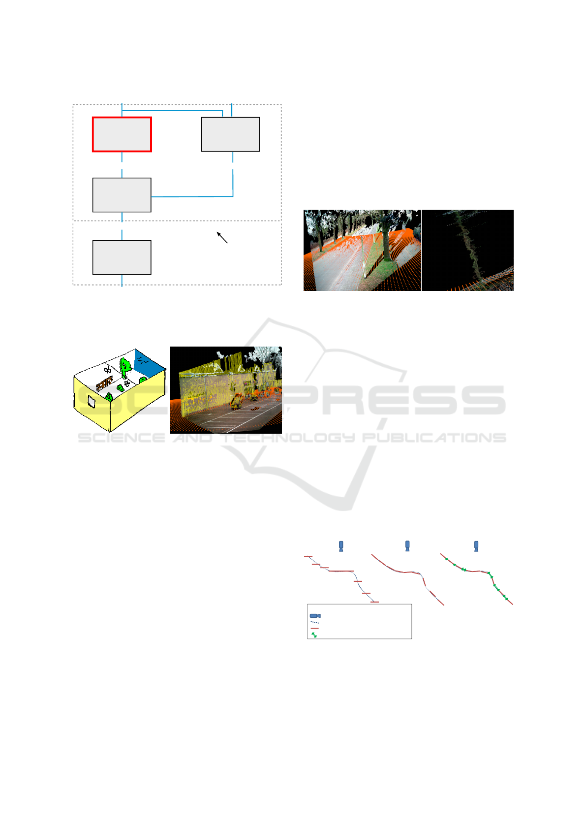
Registration

reﬁnement

Simulate live

viewpoint

Polygon model

Historic image & depth map

Live image & depth map

3D transformation [R|t]

Initial registration of historic to live image

Aligned historic and live image

3D Scene

reconstruction

Estimate 3D

transformation

Goal of this work

Figure 2: Complete overview of the 2.5D hierarchical alig-

nment approach. The red block is the focus of this paper,

where we aim at minimizing the registration error in 2D.

(a) (b)

Figure 3: (a) Diorama-box model representing the scene by

superimposing ﬂat objects on a ground plane. (b) Example

visualization of the resulting model.

4 APPROACH

We introduce a diorama-box model, as illustrated in

Figure 3, to be used as the historic 3D scene model in

the alignment approach described in Section 3. This

model is a simpliﬁcation of the real world, where ob-

jects are modeled by ﬂat planes that are perpendicular

to the optical axis. This approach is especially suited

for noisy depth data, such as captured by passive ste-

reo cameras, which is insufﬁciently accurate for con-

structing a full 3D mesh of the scene. Figure 4 shows

an example of such a point cloud as well as a zoom on

one of the trees. This ﬁgure clearly demonstrates that

it is not feasible to directly retrieve the 3D shape of

the tree. Instead, we propose to approximate all ob-

jects above the ground surface by a planar structure,

which is implemented efﬁciently by using the Stixel

World algorithm (Pfeiffer, 2012) and projecting the

stixels to 3D. In the Stixel World algorithm, the image

is ﬁrst divided into columns of ﬁxed width. Based on

the disparity estimates, each column is then split into

vertically-stacked stixels, i.e. rectangular superpixels,

using a maximum a-posteriori optimization. This pro-

cess is solved efﬁciently with dynamic programming

and results in a collection of stixels, each with a label

to contain either ground or obstacle content. In this

work, we are only interested in the obstacle stixels.

(a) (b)

Figure 4: (a) Example point cloud derived from stereo mat-

ching and (b) Zoomed view from the side of the tree, where

depth inaccuracies deform its 3D shape.

4.1 Projecting Stixels to 3D

The Stixel World algorithm results in a set of rectan-

gular super-pixels. As depth information is available,

it can be used to map these super-pixels to 3D. Ho-

wever, directly projecting each stixel to 3D causes

every stixel to be fronto-parallel, i.e. perpendicular

to the optical axis. Obviously, this might not corre-

spond to the actual orientation of the objects being

modeled. Therefore, we slant each 3D stixel to better

represent the actual objects. Stixel slanting is concep-

tually visualized in Figure 5. This slanting improves

the model accuracy when rendering to a different vie-

wpoint. The degree of slanting for each stixel is obtai-

ned through a least-squares plane ﬁt on the disparity

values within the stixel.

Top-view stixel illustration. Legend:

Camera/vehicle viewing direction

Real obstacle shape

Surface approximation with stixels

Interpolated surface stixels

A: fronto-parallel

approximation

B: slanting

C: slanting and

interpolation

Figure 5: Conceptual visualization of stixel slanting and in-

terpolation. Slanting ensures that the stixels follow the ac-

tual shape of the object more accurately, while interpolation

ﬁlls the gaps between the 3D stixels.

Fast 3D Scene Alignment with Stereo Images using a Stixel-based 3D Model

253

4.2 3D Stixel Interpolation

Although stixels connect in 2D, they do not neces-

sarily connect in 3D for two reasons. First, looking

from the camera point-of-view, camera rays diverge,

meaning adjacent pixels may map to world points,

which are far apart. Second, as each stixel is assig-

ned a slanting orientation, the stixel boundaries may

not lie at the same depth. This causes holes in the

3D model when viewed from a different camera pose,

as depicted in Figure 6(a). This ﬁgure clearly shows

that holes appear, when projecting the 3D stixels to a

different viewpoint without interpolation.

To counter this effect, we interpolate between ad-

jacent stixels as shown in Figure 5, where we add a

new stixel that connects two adjacent stixels, if they

are sufﬁciently close to each other. The effect on the

aligned image is shown in Figure 6(b).

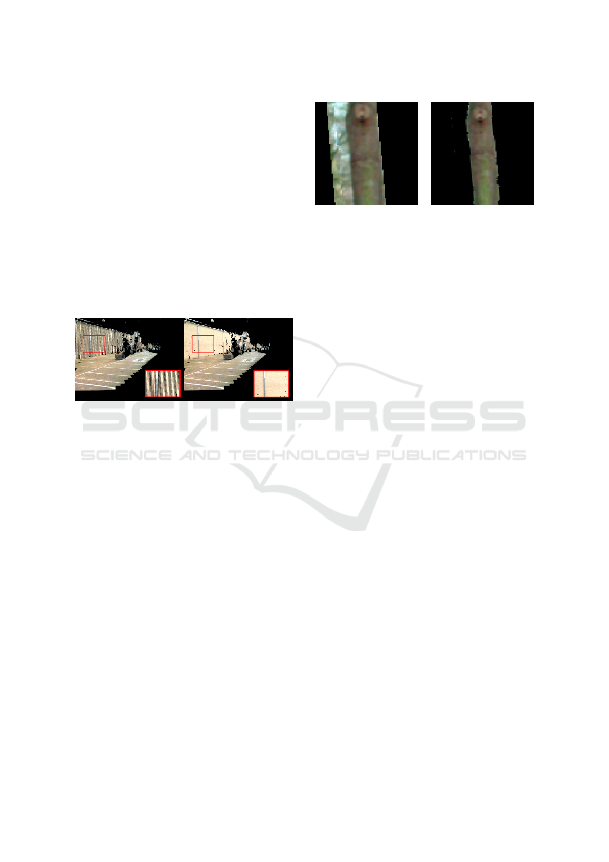
(a) (b)

Figure 6: Resulting aligned image (a) without stixel inter-

polation and (b) with stixel interpolation, when rendered to

a synthetic viewpoint.

Although computing the stixel model at a lower

resolution may decrease the number of holes in the

resulting synthesized image, this would signiﬁcantly

decrease the capability to model thin objects. The-

refore we consider the proposed stixel interpolation

better suited to reduce holes, especially because the

additional computation time is negligible.

4.3 Rejecting Invalid Pixels

In order to capture thin objects inside a stixel, we

choose thin stixels with a width of only 7 pixels. It

may still occur that an object only partially covers

a stixel, since the horizontal grid is ﬁxed. The re-

sulting stixel may therefore contain both foreground

and background pixels. Figure 7(a) shows an exam-

ple of background pixels that are incorrectly treated as

part of the tree. To correct for such errors, we adapt

the texture map prior to projecting it onto the 3D mo-

del. Here, we label all pixels inside a stixel that do not

satisfy the estimated slanting orientation, to be inva-

lid. The invalid background pixels are then removed

and replaced by black pixels in the aligned 2D image

(Figure 7(b)).

(a) (b)

Figure 7: (a) Aligned image part where background pixels

are contained inside a stixel and (b) the same image when

pixels that do not satisfy the slanting orientation are set to

invalid. This example uses wider stixels for visualization

purposes.

5 EXPERIMENTS & RESULTS

The proposed registration approach using the box-

diorama model has been validated on two separate

datasets. The ﬁrst dataset features many slanted sur-

faces, such as shown in Figure 6. The purpose of

this dataset is to speciﬁcally evaluate the added va-

lue of our stixel slanting and interpolation adaptati-

ons within the proposed registration approach. Next,

an additional dataset was recorded that features dif-

ferent lateral displacements, in order to evaluate the

effect of viewpoint differences between the live and

historic recordings.

To validate the proposed registration approach, we

evaluate it on pairs of videos, which were recorded in

both urban and industrial environments. Each video

pair features a historic recording and a live recording

of the same scene, acquired at a different moment in

time. These videos were recorded under realistic con-

ditions, by mounting the entire system on our driving

prototype vehicle. This prototype (Figure 8) features

a high-resolution stereo camera (1920 × 1440 pixels)

as well as a GPS/IMU device for accurate georefe-

rencing of all recorded images. While driving, live

and historic images featuring the same scene from dif-

ferent viewpoints are paired using GPS position and

vehicle orientation. Next, depth measurements are

obtained through disparity estimation, yielding 3D in-

formation for both the live and historic scene. At this

point, the baseline alignment approach (Section 3) is

applied, which also includes the proposed 3D scene

model (Section 4).

5.1 Performance Metrics

As this work aims at registering the live and historic

images in 2D, we measure the alignment error bet-

VISAPP 2018 - International Conference on Computer Vision Theory and Applications

254

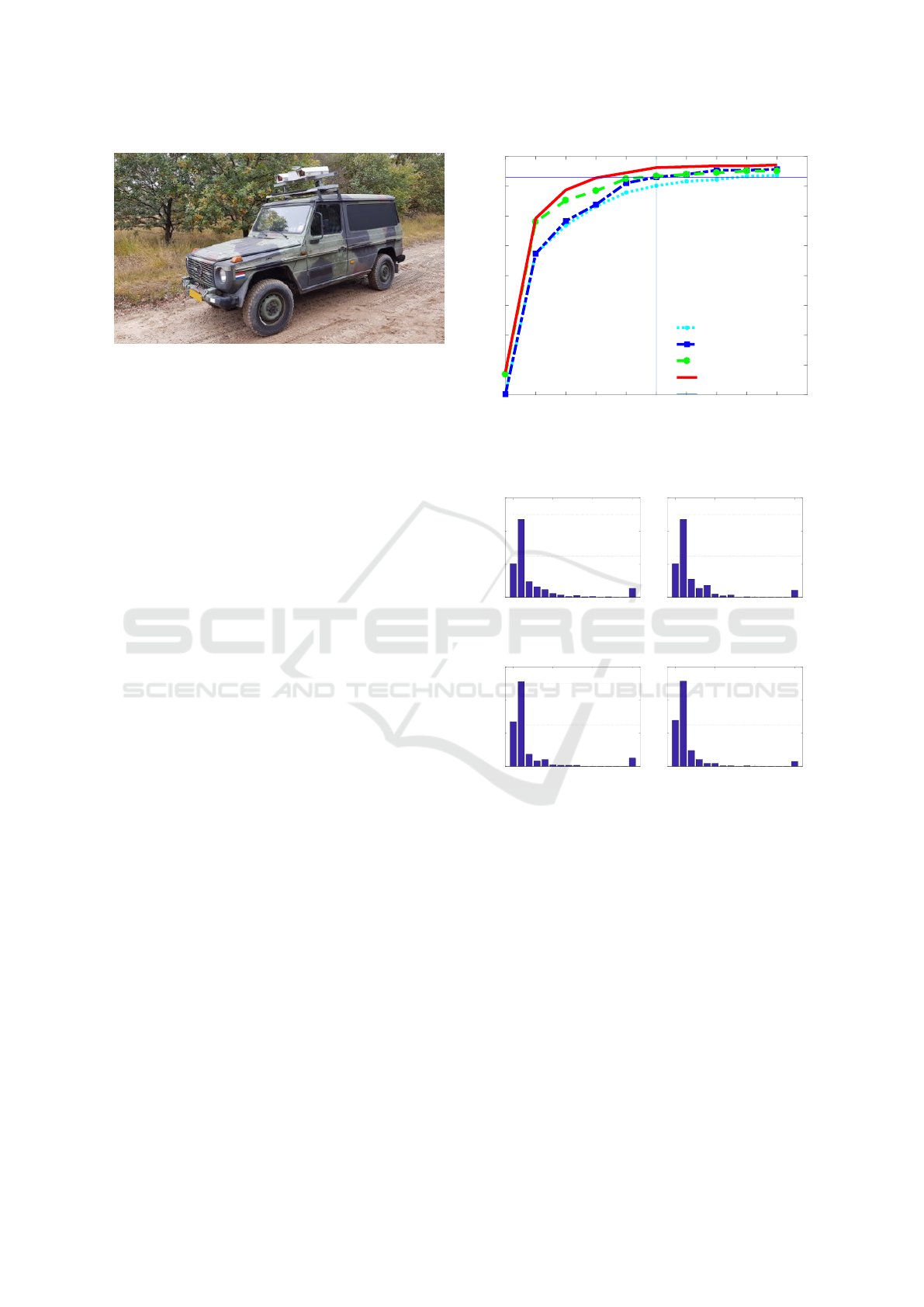
Figure 8: Prototype vehicle used for our experiments, fe-

aturing a stereo camera with 1920 × 1440 pixel resolution

and a GPS/IMU positioning system for georeferencing the

images.

ween the live image and the aligned historic image.

For the ﬁrst dataset, we have manually annotated ap-

proximately 360 characteristic points in the set of live

images, after which the exact same points were an-

notated in the registered historic images for every ex-

periment. This resulted in a total of 1,800 manually

annotated points for our ﬁrst dataset. For the second

dataset, we manually annotated 130 points for each

displacement, resulting in a total of 650 annotations

for this dataset. We employ the Euclidean distance (in

pixels) between the annotated points in the live and

registered images as a metric for the alignment accu-

racy of the proposed registration approach, including

the box-diorama model.

The registration accuracy is deﬁned as the per-

centage of annotations with an alignment error up to

5 pixels on images having 1920 × 1440 pixels. All

presented results are based on the initial registration

up to and including Stage 3 of the registration appro-

ach in Figure 2.

5.2 Evaluation

Figure 9 shows the registration accuracy when the

proposed diorama-box model is used as a 3D model

for scene alignment on our ﬁrst dataset. Even without

any post-processing, we achieve an accuracy of 90%

after initial alignment. When slanting is not consi-

dered, the stixel interpolation improves the registra-

tion accuracy from 90% to 93%. The stixel slanting

further improves the accuracy to 96%. This is also

reﬂected in Figure 10, which even shows that most

annotations have an alignment error below 2 pixels.

Moreover, Figure 9 shows that already 79% of all an-

notations have an alignment error of 1 pixel or less on

our ﬁrst dataset.

Figure 10 portrays the histograms of the alignment

errors. The reader may wonder about the 15+ pixel re-

gistration errors in the ﬁgure. These are mostly anno-

0 1 2 3 4 5 6 7 8 9

Maximum alignment error

0.2

0.3

0.4

0.5

0.6

0.7

0.8

0.9

Cumulative annotation count

original stixels

with interpolation

with slanting

with slanting and interpolation

Figure 9: Registration accuracy plotted against the maxi-

mum alignment error, showing the cumulative amount of

annotations satisfying a certain maximum alignment error.

0 5 10 15+

Alignment error (pixels)

0.2

0.4

0.6

Frequency

Alignment error histogram

(a) no slant, no interpolation

0 5 10 15+

Alignment error (pixels)

0.2

0.4

0.6

Frequency

Alignment error histogram

(b) slant, no interpolation

0 5 10 15+

Alignment error (pixels)

0.2

0.4

0.6

Frequency

Alignment error histogram

0 5 10 15+

Alignment error (pixels)

0.2

0.4

0.6

Frequency

Alignment error histogram

(d) slant and interpolation

Figure 10: Alignment error histograms when the 3D model

from Section 4 uses (a) stixels without slanting or interpo-

lation, (b) stixels with slanting but without interpolation, (c)

without slanting but with interpolation, (d) with both stixel

slanting and interpolation.

tated points that could not be registered, because that

speciﬁc part of an object was not covered by a stixel,

or because no reliable depth data was available in that

area. Such ’missing’ points are assigned to the 15+

bin.

5.3 Effect of Lateral Displacement

This experiment is performed on the second data-

set, which features different lateral displacements, i.e.

different offsets between the live and historic recor-

ding, perpendicular to the viewing direction. Such a

Fast 3D Scene Alignment with Stereo Images using a Stixel-based 3D Model

255

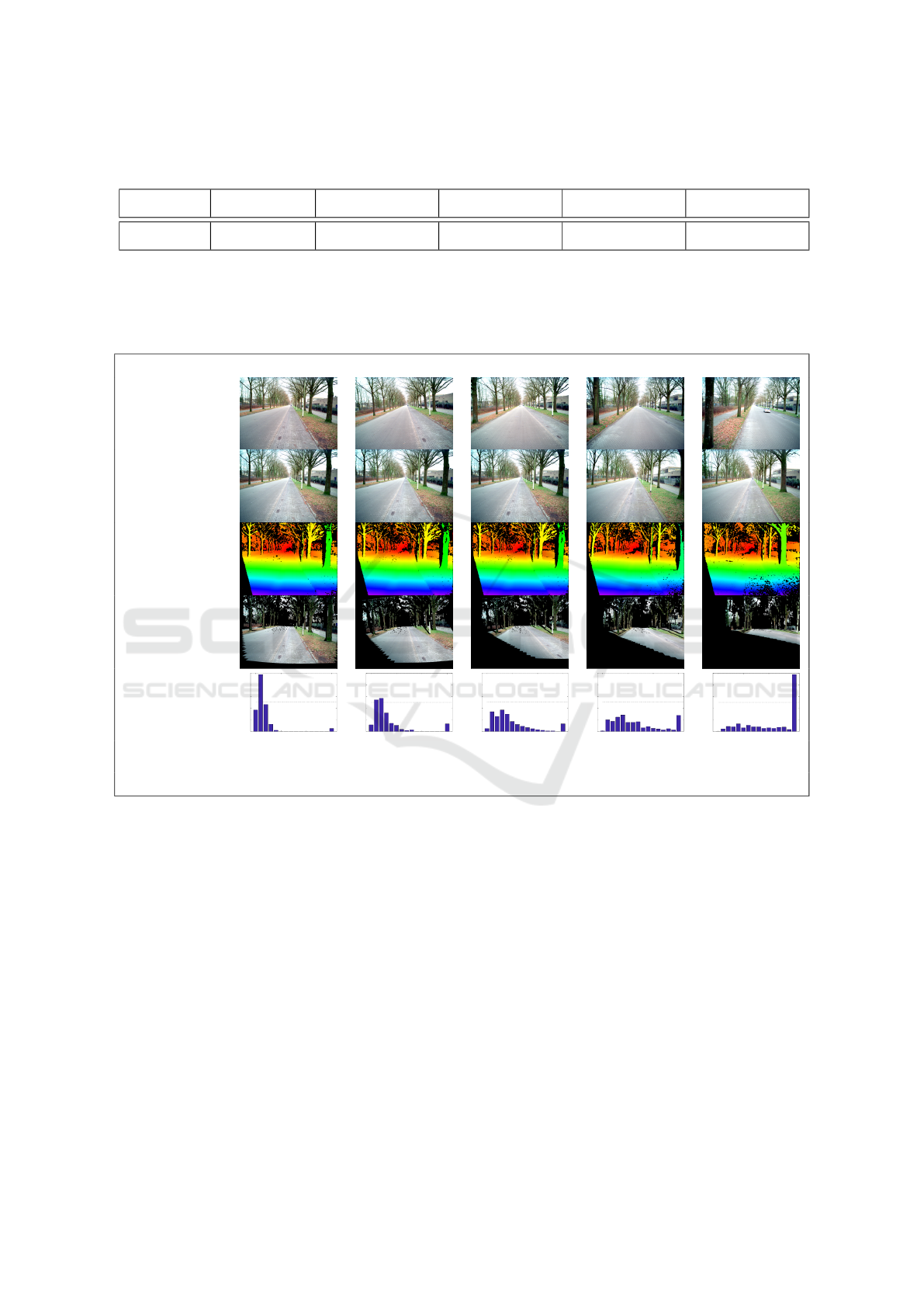
Table 1: Registration accuracy for different lateral displacements of the vehicle. In these experiments, we use annotations up

to a distance of 50 m. Figure 11 shows typical registration examples for each lateral displacement.

lateral 0cm lateral 160cm lateral 350cm lateral 530cm lateral 700cm

Proposed 97% 90% 71% 53% 20%

Table 2: Examples of the proposed registration for different lateral displacements. The ﬁrst row illustrates the target images.

The second and third row show the source images and their corresponding disparitiy maps, respectively. The fourth row

portrays the aligned images as rendered using the proposed registration approach, where black denotes areas outside of

the Field-of-View of the historic camera. Finally, the last row shows the alignment error histograms for a speciﬁc lateral

displacement using all images in the dataset with that displacement.

Live image

(target)

Historic image

(source)

Historic

disparity

Registered

image (result)

Alignment

error histogram

0 5 10 15+

Alignment error (pixels)

0.1

0.2

0.3

0.4

0.5

Frequency

0 cm

0 5 10 15+

Alignment error (pixels)

0.1

0.2

0.3

0.4

0.5

Frequency

160 cm

0 5 10 15+

Alignment error (pixels)

0.1

0.2

0.3

0.4

0.5

Frequency

350 cm

0 5 10 15+

Alignment error (pixels)

0.1

0.2

0.3

0.4

0.5

Frequency

530 cm

0 5 10 15+

Alignment error (pixels)

0.1

0.2

0.3

0.4

0.5

Frequency

700 cm

Lateral

displacement:

0 cm 160 cm 350 cm 530 cm 700 cm

lateral displacement is caused by different driving tra-

jectories between the live and historic recordings, e.g.

keeping to a different driving lane. This causes sig-

niﬁcant viewpoint differences, as shown in Figure 1.

The goal of this experiment is to identify the maxi-

mum allowed driving displacement during live opera-

tion.

Table 1 shows the registration accuracy for diffe-

rent lateral displacements for the proposed registra-

tion approach. We note that under ideal conditions,

i.e. when the live and historic driving trajectory are

almost identical, the proposed model is able to accu-

rately align 97% of all annotated points. Even at dis-

placements of 160 cm, the system is still able to align

90% of the points with an registration error of at most

5 pixels.

The decrease in registration accuracy for larger la-

teral displacements can be explained by the limited

depth accuracy of our disparity estimation algorithm,

which is outside the scope of this paper. At a distance

of 40 meters, the smallest possible disparity step cor-

responds to a jump of 25 cm. Especially at larger dis-

tances, this leads to minor inaccuracies in the depth

estimates of the stixels and hence the 3D positioning

within our scene model. This is not a problem for

small viewpoints variations (Column 2, Table 1), but

when viewed from a signiﬁcantly different viewpoint,

the objects will be projected to a different coordinate

in the registered image, i.e. will be misaligned.

The ﬁgures in Table 2 show typical examples of

the input and output of our registration framework for

different lateral displacements. Some holes in the re-

gistered images, such as part of the lantern pole mis-

sing in the second column of the table, are caused by

VISAPP 2018 - International Conference on Computer Vision Theory and Applications

256

lack of any depth estimates in that area of the disparity

map. Without depth data, no 3D object can be mo-

deled at that location. In the case of the 700-cm dis-

placement (Column 6), the only objects that remain

in the overlapping Field-of-View lie too far away to

be modeled with sufﬁcient accuracy, hence the lower

accuracy in Column 6 of Table 1.

We argue that the proposed model performs well

for small to medium lateral displacements, e.g. up

to and including 160 cm, while it is still able to align

the majority of the scene for displacements of 350 cm,

e.g. the typical distance between adjacent driving la-

nes. We note that displacements above 4 m exceed

the operational range of the proposed registration sy-

stem, although part of the scene can still be aligned

for such extreme trajectory differences. Note from Ta-

ble 2, Column 6, that the overlapping Field-of-View

of the live and historic view has become too small and

lies in the area where accurate depth information is no

longer available.

5.4 Timing

Table 3 shows the execution times of the alignment

approach when we extend the baseline method in Fi-

gure 2 with the proposed diorama-box model. Times

are shown for both separate execution and under full

CPU/GPU load, i.e. when running all pipestages si-

multaneously. Considering our HD+ stereo camera

is restricted to 6 fps, the pipelined implementation

operates at near real-time speed with 4 fps (including

scheduling overhead).

Table 3: Execution times of the proposed registration ap-

proach with the box-diorama model included. Stage 1 and

2 involve the 3D Scene reconstruction from Figure 2, while

Stage 3 both estimates the 3D transformation and simulates

the live viewpoint (Block 2 and 3 in Fig. 2). The third co-

lumn shows the execution times when the different pipeline

stages are executed simultaneously, i.e. under full load. The

(*) denotes that tasks can execute in parallel on CPU and

GPU.

t (ms)

full load

Pipelined Stage 1:

GPU: Depth estimation 90 153

Pipelined Stage 2

CPU: Ground mesh* 130 200

GPU: 3D stixels mesh* 125 160

Pipelined Stage 3

CPU: Find 3D pose diff 100 120

GPU: Viewpoint synthesis 30 46

6 DISCUSSION &

RECOMMENDATIONS

We have introduced a diorama-box model for alig-

ning images with viewpoint differences. The propo-

sed work is part of a larger change detection system

comparable to (van de Wouw et al., 2016), which aims

at ﬁnding suspicious changes in the environment of

undeﬁned shape and nature, w.r.t. a previous recor-

ding. Scene alignment is a crucial aspect of this sy-

stem, since without proper alignment the scene can-

not be compared and changes may be missed. By

extending the 3D ground-surface model of the base-

line system with 3D objects, the operational range of

the change detection system is signiﬁcantly improved,

where the analysis is no longer limited to the ground

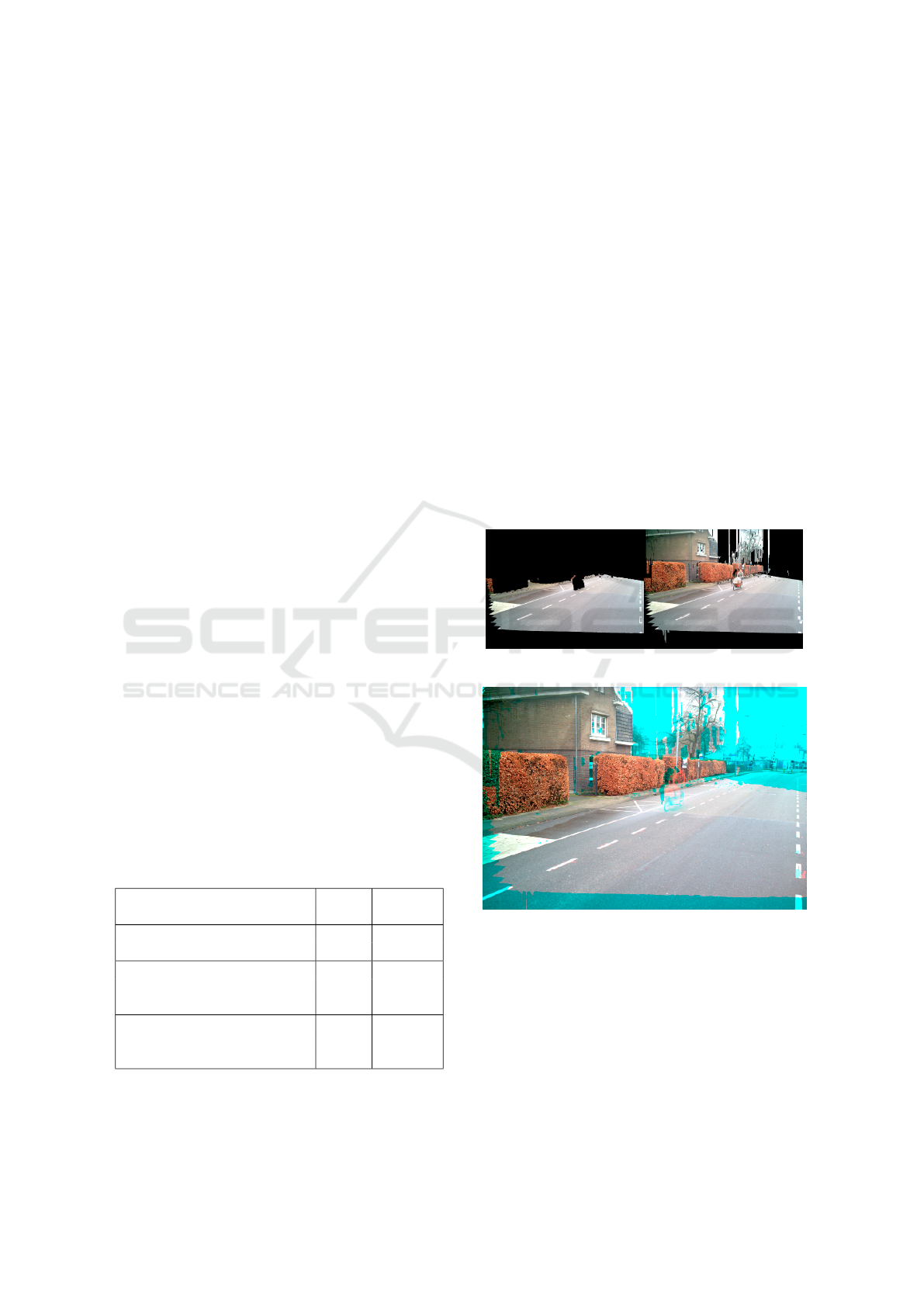
surface. Figure 11 shows the aligned images with and

without the proposed model, clearly showing the im-

proved alignment coverage, i.e. a larger part of the

scene can be exploited for change detection.

(a) (b)

(c)

Figure 11: Aligned images when using (a) ground-surface

model from (van de Wouw et al., 2016), (b) proposed model

including the 3D objects. Subﬁgure (c) shows an overlay of

the live image (cyan) and the aligned historic scene (red).

Although the proposed work has similarities with

the multi-view registration approaches discussed in

Section 2, we cannot use the datasets introduced in

their work. These datasets typically feature mono

images from different viewpoint, whereas we need

stereo images or a disparity map in our approach.

Fast 3D Scene Alignment with Stereo Images using a Stixel-based 3D Model

257

It was observed that rejecting invalid pixels within

stixels occasionally results in small holes in the regis-

tered images at locations where no disparity estimate

is available. Although such holes can mostly be avoi-

ded by using a morphological-closing ﬁlter prior to

rejecting the pixels, some holes may persist. Howe-

ver, the downside of having small holes in the registe-

red image did not outweigh the beneﬁt of having a cle-

aner texture projection. We plan to look into guided-

image ﬁltering to prevent such holes and further reﬁne

the stixel boundaries in future work.

The current disparity estimation, which is outside

the scope of this work, is noisy and has a very limited

sub-pixel resolution. We hypothesize that a more ex-

pensive disparity estimation algorithm, increased ba-

seline or zoom-lenses will improve the depth accu-

racy, which in turn will extend the operational range

of the proposed 3D model.

7 CONCLUSION

We have introduced a diorama-box model for aligning

images acquired from a moving vehicle. The propo-

sed model extends the non-linear ground surface mo-

del (van de Wouw et al., 2016) with a model of the

3D objects in the scene. For this purpose, the Stixel

World algorithm is used to segment the scene into

super-pixels, which are projected to 3D to form an

obstacle model. The consistency of the stixel-based

model is improved by assigning a slanting orienta-

tion to each 3D stixel and by interpolating between

the stixels to ﬁll gaps in the 3D model. Conse-

quently, registration accuracy is increased by 6%. As

a further improvement of the algorithm, background

pixels contained in object-related stixels are removed

by checking their consistency with the stixel-slanting

orientation. This improvement prevents ghosting ef-

fects, due to falsely projected background pixels.

The resulting alignment framework shows good

results for typical driving scenarios, in which both

live and historic recordings were acquired from the

same driving lane. In this case, 96% of all manu-

ally annotated points are registered with an alignment

error up to 5 pixels for images with a resolution of

1920 × 1440 pixels, where even 79% of the annotati-

ons have an error of unity pixel or lower. Even when

driving in an adjacent lane, the system is able to accu-

rately align 71% of all annotated points.

It was found that the disparity resolution of the

depth map, i.e. the lack of sub-pixel accuracy, limits

the accuracy of the 3D model, making it less effective

for displacements above 4 meters. Nevertheless, the

proposed work signiﬁcantly improves the operatio-

nal range of the real-time change detection system,

which now covers the full 3D scene, instead of only

the ground plane. Higher accuracies and/or perfor-

mance of the change detection system can be achie-

ved when important parameters are improved, such as

lenses and/or a larger baseline, together with a more

accurate depth estimation algorithm.

REFERENCES

Achanta, R., Shaji, A., Smith, K., Lucchi, A., Fua, P., and

Susstrunk, S. (2012). Slic superpixels compared to

state-of-the-art superpixel methods. IEEE Trans. Pat-

tern Anal. Mach. Intell., 34(11):2274–2282.

Broggi, A., Cattani, S., Patander, M., Sabbatelli, M., and

Zani, P. (2013). A full-3d voxel-based dynamic ob-

stacle detection for urban scenario using stereo vi-

sion. In Intelligent Transportation Systems-(ITSC),

2013 16th International IEEE Conference on, pages

71–76. IEEE.

Chauve, A. L., Labatut, P., and Pons, J. P. (2010). Ro-

bust piecewise-planar 3d reconstruction and comple-

tion from large-scale unstructured point data. In 2010

IEEE Computer Society Conference on Computer Vi-

sion and Pattern Recognition, pages 1261–1268.

Cordts, M., Rehfeld, T., Enzweiler, M., Franke, U., and

Roth, S. (2016). Tree-structured models for efﬁcient

multi-cue scene labeling. IEEE Transactions on Pat-

tern Analysis and Machine Intelligence.

Felzenszwalb, P. F. and Huttenlocher, D. P. (2004). Efﬁ-

cient graph-based image segmentation. International

Journal of Computer Vision, 59(2):167–181.

Labatut, P., Pons, J.-P., and Keriven, R. (2009). Robust and

efﬁcient surface reconstruction from range data. In

Computer graphics forum, volume 28, pages 2275–

2290. Wiley Online Library.

Lou, Z. and Gevers, T. (2014). Image alignment by piece-

wise planar region matching. IEEE Transactions on

Multimedia, 16(7):2052–2061.

Maiti, A. and Chakravarty, D. (2016). Performance analy-

sis of different surface reconstruction algorithms for

3d reconstruction of outdoor objects from their digital

images. SpringerPlus, 5(1):932.

Natour, G. E., Ait-Aider, O., Rouveure, R., Berry, F., and

Faure, P. (2015). Toward 3d reconstruction of outdoor

scenes using an mmw radar and a monocular vision

sensor. Sensors, 15(10):25937–25967.

Pfeiffer, D.-I. D. (2012). The stixel world. PhD thesis,

Humboldt-Universit

at zu Berlin.

Salman, N. and Yvinec, M. (2010). Surface reconstruction

from multi-view stereo of large-scale outdoor scenes.

International Journal of Virtual Reality, 9(1):19–26.

Sanberg, W. P., Do, L., and de With, P. H. N. (2013). Flex-

ible multi-modal graph-based segmentation. In Ad-

vanced Concepts for Intelligent Vision Systems: 15th

International Conference, ACIVS 2013, Pozna

n, Po-

land, October 28-31, 2013. Proceedings, pages 492–

503. Springer International Publishing.

VISAPP 2018 - International Conference on Computer Vision Theory and Applications

258

Strom, J., Richardson, A., and Olson, E. (2010). Graph-

based segmentation for colored 3d laser point clouds.

In Intelligent Robots and Systems (IROS), 2010

IEEE/RSJ International Conference on, pages 2131–

2136. IEEE.

Su, H. R. and Lai, S. H. (2015). Non-rigid registration of

images with geometric and photometric deformation

by using local afﬁne Fourier-moment matching. Pro-

ceedings of the IEEE Computer Society Conference

on Computer Vision and Pattern Recognition, 07-12-

June:2874–2882.

van de Wouw, D. W. J. M., Dubbelman, G., and de With,

P. H. N. (2016). Hierarchical 2.5-d scene alignment

for change detection with large viewpoint differences.

IEEE Robotics and Automation Letters, 1(1):361–368.

van de Wouw, D. W. J. M., Pieck, M. A., Dubbelman, G.,

and de With, P. H. (2017). Real-time estimation of

the 3d transformation between images with large vie-

wpoint differences in cluttered environments. Electro-

nic Imaging, 2017(13):109–116.

Veksler, O., Boykov, Y., and Mehrani, P. (2010). Super-

pixels and supervoxels in an energy optimization fra-

mework. In European conference on Computer vision,

pages 211–224. Springer.

Werlberger, M., Pock, T., and Bischof, H. (2010). Mo-

tion estimation with non-local total variation regula-

rization. In 2010 IEEE Computer Society Conference

on Computer Vision and Pattern Recognition, pages

2464–2471.

Yamaguchi, K., McAllester, D., and Urtasun, R. (2014). Ef-

ﬁcient Joint Segmentation, Occlusion Labeling, Stereo

and Flow Estimation, pages 756–771. Springer Inter-

national Publishing, Cham.

Zhang, G., He, Y., Chen, W., Jia, J., and Bao, H. (2016).

Multi-Viewpoint Panorama Construction with Wide-

Baseline Images. IEEE Transactions on Image Pro-

cessing, 25(7):3099–3111.

Fast 3D Scene Alignment with Stereo Images using a Stixel-based 3D Model

259