
Qualitative Simulation of Hybrid Systems with an Application to SysML
Models
Slim Medimegh
1
, Jean-Yves Pierron
1
and Frédéric Boulanger
2
1
CEA LIST, Laboratory of Model Driven Engineering for Embedded Systems, P.C. 174, 91191 Gif-sur-Yvette, France
2
LRI, CentraleSupélec, Université Paris-Saclay, 3 rue Joliot-Curie, 91192 Gif-sur-Yvette, France
Keywords:
Hybrid Systems, Qualitative Simulation, Symbolic Execution, Model Transformation.
Abstract:
Hybrid systems are specified in a heterogeneous form, with discrete and continuous parts. Simulating such
systems requires precise data and synchronization of continuous changes and discrete transitions. However, in
the early design stages, missing information forbids numerical simulation. We present here a symbolic execu-
tion model for the qualitative simulation of hybrid systems, which consists in computing only qualities of the
behavior. This model is implemented in the Diversity symbolic execution engine to build the qualitative be-
haviors of the system. We apply this approach to the analysis of SysML models, using an M2M transformation
from SysML to a pivot language and an M2T transformation from this language to Diversity.
1 INTRODUCTION
Embedded software has become essential in most in-
dustrial sectors, leading to heterogeneous models of
a whole system, with discrete and continuous parts.
Simulating such hybrid systems requires precise data
and computational power for detecting changes in the
continuous values and synchronizing them with dis-
crete transitions. However, in the early stages of the
design, the exact value of some parameters is not
known yet, while it is already necessary to analyze
the behavior of the system to make design decisions.
For continuous variables, the laws of evolution are
often described by differential equations. Qualitative
simulation can be an alternative to numerical simula-
tion for such models. Its principle is the discretiza-
tion of the domain of variation of the continuous vari-
ables and their derivatives, leading to a qualitative de-
scription of their evolution: positive, negative, null,
increasing, decreasing, constant, at a maximum etc.
In this way, one can get a tree of abstract behaviors,
each node describing the qualitative evolution of the
variables during a phase of the behavior. Combined
with a model of the discrete part of the system, this
yields a discrete model of the behavior of the whole
system to which formal techniques can be applied.
When the exact differential equations are not
known, an abstract qualitative model of the laws of
evolution of the continuous variable, described as an
automaton, can be used.
In this article, we present a new symbolic execu-
tion model for qualitative simulation, which relies on
a qualitative model of the continuous behavior of the
system, and on symbolic integration of the first two
derivatives of the state variables. This model of exe-
cution is implemented in the Diversity (Rapin et al.,
2003) tool in order to compute the qualitative be-
havior of hybrid systems. We use SysML to model
the qualitative behavior of our system, and model
driven engineering techniques such as QVT opera-
tional and Acceleo in order to have a complete tool
chain that takes a SysML model and produces a Di-
versity model.
This article has two main parts: in the first one, we
present the context of our work and our symbolic exe-
cution model for qualitative simulation, in the second
part we present how to use SysML in this context.
2 QUALITATIVE SIMULATION
Hybrid Dynamic Systems consist of continuous dy-
namic systems, discrete event systems and interaction
between both types of systems (Lynch et al., 2003).
Such systems result from the hierarchical organiza-
tion of monitoring/control systems, or from the inter-
action between algorithms for discrete planning and
continuous control. These systems can be modeled
using hybrid automata, which are defined by a set of
Medimegh, S., Pierron, J-Y. and Boulanger, F.
Qualitative Simulation of Hybrid Systems with an Application to SysML Models.
DOI: 10.5220/0006535202790286
In Proceedings of the 6th International Conference on Model-Driven Engineering and Software Development (MODELSWARD 2018), pages 279-286
ISBN: 978-989-758-283-7
Copyright © 2018 by SCITEPRESS – Science and Technology Publications, Lda. All rights reserved
279

continuous variables and states, and discrete transi-
tions with guards and assignments to these variables.
Qualitative Simulation. comes from artificial in-
telligence, where it is used for reasoning about contin-
uous aspects of systems. The goal is to reason about
the behavior of a continuous variable without com-
puting its value. For hybrid systems, the model of
the discrete part of the system is not changed by the
qualitative abstraction process. However, continuous
variables and their derivatives are discretized in order
to consider only their qualitative changes. Therefore,
continuous behaviors become discrete transitions, and
the resulting system allows behaviors that are disal-
lowed by the actual physics. However, it may overap-
proximate (in a safe way) the possible behaviors.
The Principle of Qualitative Simulation. is the
discretization by partitioning the variation range of
the continuous variables of the system and their
derivative to compute their qualitative state (increas-
ing, decreasing, constant etc.) This principle can
be extended to the n
th
derivative to distinguish more
qualitative states. Once the discrete states correspond-
ing to this qualitative partitioning are created, we
build the possible transitions by taking into account
continuity and derivative constraints. For instance,
each variable or derivative can not go from negative
to positive without going through zero, and a variable
can go from negative to zero or from zero to positive
only if its derivative is positive etc. Finally, the differ-
ential equation system is abstracted into a transition
system whose states are based on the partitioning of
the changes of continuous variables and derivatives,
and whose transitions are the physically possible evo-
lutions between these states. The result of the quali-
tative simulation is an abstraction of the solutions to
the differential equations system.
Diversity. is a symbolic execution engine devel-
oped at CEA LIST to produce symbolic scenarios cor-
responding to classes of system behaviors. These sce-
narios are used to prove properties and to generate
concrete numerical tests. To guarantee termination or
to limit the number of generated test cases, the size
and the number of behaviors can be bounded, and re-
dundant behavior detection can be used.
Diversity can be used for qualitative simulation
according to two strategies (Gallois and Pierron,
2016): qualitative simulation with differential equa-
tions, and qualitative simulation without differential
equations. In the first approach, the differential equa-
tions are known, and the QEPCAD tool (Brown,
2003) is used to determine the conditions for a qual-
itative change. When a change is possible, the cor-
responding branch is tagged with the conditions, else
the corresponding branch in the execution tree is cut.
In the second approach, the differential equations
are not available or it is too difficult to deal with their
complexity. In this case, we build a qualitative model
of the equations by considering qualitative relations
between the variables and their derivatives. Of course,
the results are less precise than in the first approach,
but this can be used at very early stages of the de-
sign. In this article, we deal with this second ap-
proach. We therefore use Diversity to symbolically
execute the model of a hybrid system, which com-
bines the model of its discrete part and the discretized
qualitative model of its continuous part.
Symbolic Execution in Diversity is performed by
assigning symbolic values to variables instead of nu-
merical ones, and yields symbolic states named exe-
cution contexts. As illustrated in Figure 1, an execu-
tion context includes: (1) a Control State; (2) a Path
Condition, which is the condition to reach the sym-
bolic state from the initial state; (3) a symbolic mem-
ory which associates to each variable an expression
based on symbolic inputs.
The result of a symbolic execution is an execution
tree where each path represents the symbolic evolu-
EC =
CS : Null_der
PC : ˙x]
1
= 0
¨x
-1
= ¨x
-1
]
0
˙x = ˙x]
1
vspace0.10cm
Figure 1: Execution Context.
Null_der
Pos_der
Neg_der
t
1
:
¨x
-1
> 0
˙x
-1
← ˙x
˙x ← ˙x
-1
+ ¨x
-1
t
2
:
¨x
-1
< 0
˙x
-1
← ˙x
˙x ← ˙x
-1
+ ¨x
-1
Figure 2: Transititons.
EC
1
=
CS : Pos_der
PC : ˙x]
1
= 0 ∧ ¨x
-1
]
0
> 0
˙x
-1
= ˙x]
1
˙x = ˙x]
1
+ ¨x
-1
]
0
EC
2
=
CS : Neg_der
PC : ˙x]
1
= 0 ∧ ¨x
-1
]
0
< 0
˙x
-1
= ˙x]
1
˙x = ˙x]
1
+ ¨x
-1
]
0
Figure 3: Symbolic Execution.
MODELSWARD 2018 - 6th International Conference on Model-Driven Engineering and Software Development
280

tion of the variables. The path condition is the con-
junction of all the execution conditions. The ] nota-
tion is used to index successive symbolic values.
Figure 2 shows transitions t
1
and t
2
from source
state Null_der, the control state of the execution con-
text EC of Figure 1. The symbolic execution of t
1
and
t
2
produces two execution contexts described in Fig-
ure 3, which correspond to the two possible behaviors.
2.1 Related Work
Kuipers’ algorithm for qualitative simulation,
QSIM (Kuipers, 1986), is based on an algebra of
signs. Numerous improvements have been added to
QSIM in order to address the combinatory explosion
of the number of predicted states:
• Methods for changing the level of description in
order to eliminate behaviors with no qualitative
distinctions (Kuipers and Chiu, 1987).
• Reasoning on “high order derivative” to provide
a curvature constraints (Kuipers and Chiu, 1987)
(de Kleer and Bobrow, 1984).
• Adding energy constraint that decomposes the
system into a conservative part and a non conser-
vative one (Fouché and Kuipers, 1992).
However, some problems such as obtaining and us-
ing adequate temporal information still remain. This
problem was approached in (Shen and Leitch, 1990)
and (Berleant and Kuipers, 1992). The most famous
tool for qualitative simulation is Garp3 (Bredeweg
et al., 2009). It runs model fragments, which describe
part of the structure and behavior of the system, and
produces a state graph which contains all the possible
transitions based on the relationships between entities
that are described in the model fragments.
However, the problem we address is how to
predict the qualitative behavior of continuous vari-
ables of hybrid systems without differential equa-
tions. (Bredeweg et al., 2009) describes the variation
of the second derivative as small arrows and dots next
to the derivative symbol. From a user point of view, it
is not easy to analyze the behaviors generated by this
simulator, that is why we propose to compute the dif-
ferent qualitative states by taking into consideration
the second and first derivatives. (Missier and Trave-
Massuyes, 1991) proposed a temporal filter based on
order of magnitude representation and second order
Taylor formula to evaluate the duration for qualitative
states, but we are not interested in temporal informa-
tion because we are in the first steps of the design;
time is not critical at this stage. We therefore rely
on a qualitative symbolic integration with the Euler
method, assuming a unitary integration step. In order
to eliminate the indeterminacy problem of the algo-
rithm of (Kuipers, 1986), our model of execution is
based on symbolic values.
2.2 A New Symbolic Execution Model
For improving the qualitative simulation without dif-
ferential equations in Diversity, we developed a model
of execution that constraints the evolution of the state
variables, and computes their qualitative behavior.
= 0
> 0< 0
der = 0
der > 0
der < 0
der < 0
der > 0
Figure 4: Qualitative changes.
= 0
x
-1
← x
x ← x
-1
+ ˙x
-1
< 0
x
-1
← x
x ← x
-1
+ ˙x
-1
> 0
x
-1
← x
x ← x
-1
+ ˙x
-1
˙x
-1
< 0 ˙x
-1
> 0
˙x
-1
> 0 and
˙x
-1
= −x
˙x
-1
< 0 and
˙x
-1
= −x
( ˙x
-1
< 0) or
( ˙x
-1
> 0 and ˙x
-1
< −x)
( ˙x
-1
> 0) or
( ˙x
-1
< 0 and ˙x
-1
> −x)
Figure 5: Qualitative changes based on symbolic integra-
tion.
Model of Execution. In our previous work (Med-
imegh et al., 2016), we presented a qualitative model
of execution with continuity and derivative con-
straints for the changes of the state variables. For
instance, the value of a state variable cannot change
from Negative to Positive without being Null, and it
cannot change from Negative to Null unless the first
derivative is positive. The same rules apply to the first
derivative with regard to the second derivative. These
constraints can be modeled in a state machine as illus-
trated in Figure 4. A similar automaton controls the
changes of the first derivative. Unfortunately, these
state machines are nondeterministic. For instance, in
the > 0 state, if the first derivative is Negative, we can
either go to the = 0 state or stay in the current state.
In this paper, we present a new symbolic execu-
tion model in which we integrate the derivatives of
Qualitative Simulation of Hybrid Systems with an Application to SysML Models
281

the state variables in a symbolic way. We use a sim-
ple Euler integration since we do not compute exact
numerical values. We model each continuous state
variable by six values: the current (x) and previous
(x
-1
) values of the variable, the current ( ˙x) and previ-
ous ( ˙x
-1
) values of its first derivative, and its current
second derivative ( ¨x). In this new model of execution,
we add the previous second derivative ( ¨x
-1
), which is
needed to integrate the first derivative. The symbolic
integration with the Euler method, assuming a unitary
integration step gives x = x
-1
+ ˙x
-1
, and ˙x = ˙x
-1
+ ¨x
-1
.
With these rules, the qualitative value of a state
variable is controlled by a state machine as illustrated
in Figure 5. A similar automaton controls the change
of the first derivative with respect to its previous value
( ˙x
-1
) and the previous second derivative ( ¨x
-1
). Con-
trary to our previous work, these state machines are
deterministic. For instance, in the > 0 state of x, if ˙x
-1
< 0 and ˙x
-1
= -x
-1
, we go to the = 0 state, if ˙x
-1
> 0 or
˙x
-1
< 0 and - ˙x
-1
< x, we stay in the current state.
Implementation of Our Execution Model in Diver-
sity. This execution model with symbolic integra-
tion relies on five automata: the first one is the sys-
tem automaton in which the user models his system
and specifies the different values of the current second
derivative; the second automaton keeps track of the
qualitative value of the second derivative ( ¨x), which
is driven by the system automaton; the third automa-
ton keeps track of the qualitative value of the first
derivative ( ˙x), which is symbolically integrated from
the previous first and second derivatives; the fourth
automaton keeps track of the qualitative value of the
state variable (x), which is symbolically integrated
from the previous value and first derivative; and fi-
nally, the fifth automaton computes the qualitative
variation of the variable by observing the automata
for the qualitative value of the variable, its derivatives,
and their previous value.
The order in which these automata are executed
is important: we execute the automaton of the sys-
tem first, then the automaton for the second deriva-
tive, then the automaton for the first derivative, then
the automaton for the value of the state variable, and
finally the automaton for the qualitative behavior.
Computing Second Order Qualitative Behaviors.
In our previous work (Medimegh et al., 2016), we
showed how to compute the qualitative behavior of a
state variable by observing the qualitative state of this
variable and its derivatives. For instance, when the
second derivative is Negative and the first derivative
is Null, with a Positive previous derivative, we have
the qualitative behavior Maximum.
With that qualitative model, we identified 13 qual-
itative states of behavior: Constant when ˙x
-1
, ˙x and
¨x are null; FlexStartIncrease when ˙x
-1
= 0, ˙x = 0
and ¨x > 0, so the first derivative is not positive yet,
but the dynamics is transitioning toward an increase;
FlexStartDecrease when ˙x
-1
= 0, ˙x = 0 and ¨x < 0,
which is similar to the previous case when transition-
ing toward a decrease; StartIncrease when ˙x
-1
= 0
and ˙x > 0, the first derivative has just become posi-
tive (notice that there is no condition on the second
derivative, which may have come back to 0); Start-
Decrease when ˙x
-1
= 0 and ˙x < 0; Increase when
˙x
-
1
> 0 and ˙x > 0, the first derivative being positive;
Decrease when ˙x
-1
< 0 and ˙x < 0, the first derivative
being negative; Maximum when ˙x
-1
> 0, ˙x = 0 and
¨x < 0, the three conditions are necessary to distin-
guish this case from other qualitative states such as
inflection points; Minimum when ˙x
-1
< 0, ˙x = 0 and
¨x > 0, same remark as for the Maximum; FlexIn-
crease when ˙x
-1
> 0, ˙x = 0 and ¨x > 0, an inflection
point during an increase; FlexDecrease when ˙x
-1
< 0,
˙x = 0 and ¨x < 0, an inflection point during a decrease;
StopIncrease when ˙x
-1
> 0, ˙x = 0 and ¨x = 0, the state
variable reaches a plateau at the end of an increase;
StopDecrease when ˙x
-1
< 0, ˙x = 0 and ¨x = 0, the state
variable reaches a plateau at the end of a decrease.
By additionally taking into account x
-1
and x, it is
possible to distinguish sub-cases in these qualitative
states, for instance “reaching a null maximum” when
reaching a maximum with x
-1
< 0 and x = 0.
There are impossible cases. Two are due to the
continuity of the variable: the conjunction of x
-1
< 0
and x > 0, and the conjunction of x
-1
> 0 and x < 0 are
impossible. Two others are due to the continuity of
the first derivative (no angular points). Ten others are
due to the fact that each variable change is constrained
by the previous value of its first derivative.
In the new model of execution, we add qualita-
tive states to model higher order qualitative variations,
which qualify the variation of the first derivative: In-
creasingly_Increase, when ˙x
-1
> 0 and ¨x
-1
> 0; De-
creasingly_Increase when ˙x
-1
> 0 and ¨x
-1
< 0; In-
creasingly_Decrease, when ˙x
-1
< 0 and ¨x
-1
< 0; De-
creasingly_Decrease when ˙x
-1
< 0 and ¨x
-1
> 0.
Illustrative Example of the Bouncing Ball. This
technique was applied to the bouncing ball, a typical
example of hybrid system. In this example, we have
only one state variable, the height of the ball above the
ground, noted z. The usual way to model the bouncing
ball is to consider that it has only one state, in which
it is in free fall, with ¨z = −g and g = 9.81m.s
−2
. The
bounce is modeled with a single transition, which is
triggered when the ball hits the ground (z = 0), and
MODELSWARD 2018 - 6th International Conference on Model-Driven Engineering and Software Development
282
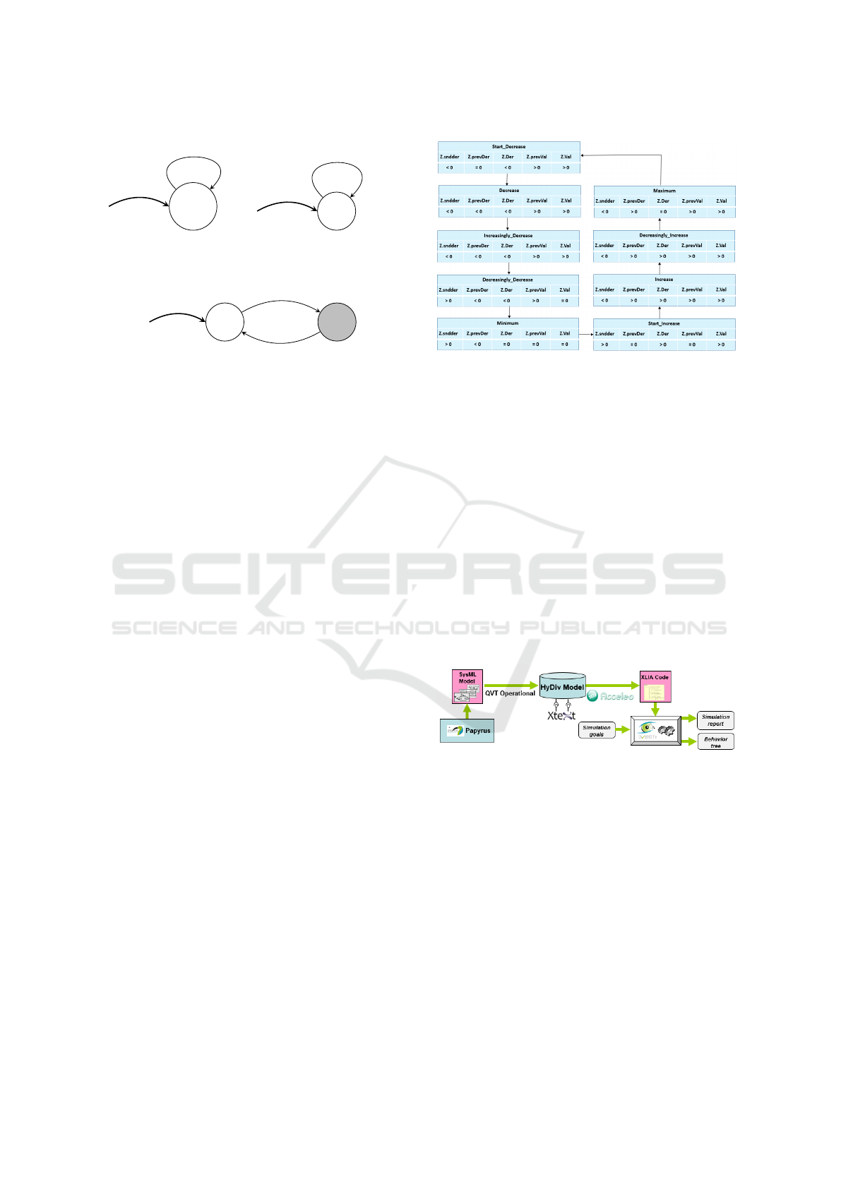
¨z = −g
z = 0 / ˙z = −c.˙z
z > 0
˙z = 0
¨z < 0
z = 0 / ˙z = −˙z
z > 0
˙z = 0
Figure 6: Hybrid (left) and qualitative (right) automata of
the bouncing ball.
¨z < 0 ¨z > 0
z > 0
˙z = 0
z = 0
z > 0
Figure 7: Adjusted Model for the Bouncing Ball.
reverses the speed of the ball with a damping factor
0 < c ≤ 1. This model and its qualitative abstraction
are shown in Figure 6.
The quantitative behavior of this model is an ab-
straction of what really happens, because if the ball
were really changing its speed instantaneously, there
would be an exchange of a finite amount of energy
in zero time between the ball and its environment,
which corresponds to an infinite power. We have
shown (Medimegh et al., 2016) that in the case of
the bouncing ball, the model can be automatically ad-
justed by replacing the bouncing transition by a series
of transitions. The algorithm for this is as follows:
• changing the derivative from < 0 to > 0 is illegal.
The only legal path is to go from < 0 to = 0 and
then from = 0 to > 0, so we replace the illegal
transition by a legal one.
• changing the derivative from < 0 to 0 and from
0 to > 0 requires a positive second derivative, so
we make it positive during the bounce (the second
derivative can be discontinuous).
The resulting state machine is shown in Figure 7,
where the additional state has a gray background.
The additional state, reached when z = 0, sets the
second derivative to Positive because this is required
to make the first derivative change from Negative to
Null. When the first derivative becomes null, our new
symbolic execution model finds a path to make the
first derivative positive because the second derivative
is still positive. The velocity of the ball becomes then
positive, as requested by the initial un-physical tran-
sition, we can go back to the free fall state of the ball,
with a reversed velocity.
With this adjusted model and the symbolic execu-
tion model for qualitative simulation, we obtain the
qualitative behavior shown in Figure 8.
Figure 8: Qualitative behavior of the bouncing ball.
3 SysML MODELS
To make our approach usable for system designers,
and to insulate them from changes in our execution
model and input format, we built a tool chain to use
SysML as input for qualitative simulation. We choose
SysML because it allows the modeling of multi do-
main specifications. It is also used by a large com-
munity of engineers to model the system at the early
design stages.
Our approach relies on a qualitative model of
the continuous behavior, not on the exact differen-
tial equations. This qualitative model is already dis-
cretized, so we can use the state machines diagram to
model the behavior of the hybrid system.
Figure 9: The Tool Chain.
3.1 Presentation of the Tool Chain
We model a hybrid system with a SysML state ma-
chine diagram, using the Papyrus Eclipse plug-in.
Then, we transform the SysML model using a QVT
operational model to model transformation into a Hy-
Div model. HyDiv is a pivot meta-model that we de-
signed to capture a high level representation of the hy-
brid system, independently of the source model (we
could use Simulink/Stateflow instead of SysML). We
then use an Acceleo model to text transformation to
transform the HyDiv model into Xlia, the input lan-
guage of Diversity, as shown in Figure 9.
Qualitative Simulation of Hybrid Systems with an Application to SysML Models
283
The SysML Model. The hybrid system is modeled
as a SysML Block with attributes for the variables and
the behavior of the system. The variables have the
Derivative_Type and the behavior is defined by a State
Machine. In this state machine, the guards are writ-
ten in OCL. We specify the Effect of a transition by
a Specification to which we attach an Operation with
an OCL constraint. We use the same technique for the
Entry actions of the states.
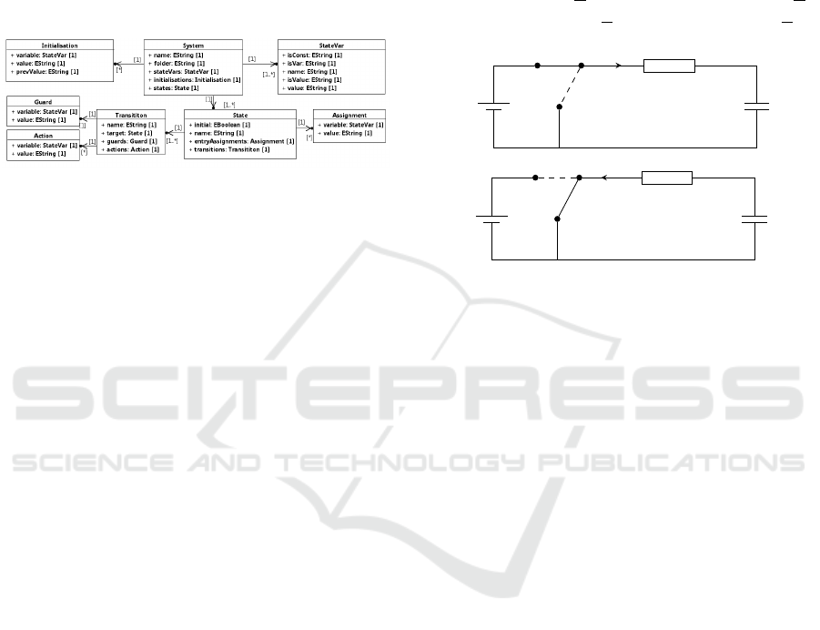
Figure 10: The HyDiv Metamodel.
The HyDiv Model. HyDiv is a textual domain spe-
cific modeling language for hybrid systems, imple-
mented with Xtext. It provides us with a compact
representation of the system which is decoupled from
both the input formalism (SysML in this article) and
the model of execution that will be used in Diversity.
Figure 10 shows its meta-model, in which the system
has different attributes: a name, a folder to indicate
its location, statesVars to indicate its state variables,
initializations to indicate the initial value of the vari-
ables, and states to describe the states of the hybrid
system. Each State has an initial attribute, a name,
entryAssignments to describe the actions to perform
when entering the state, and transitions toward other
states. Each Transition has a name, a target state,
guards to tell when the transition can be fired, and
actions to be performed by the transition.
QVT Operational Transformation. The first step
to perform the qualitative simulation of a system is to
transform its SysML model into HyDiv. The QVT
operational transformation from SysML to HyDiv
makes the following mappings:
• a SysML Block is mapped to System;
• an Attribute of a block with Derivative_Type or
Integer as type is mapped to StateVar;
• a State of a state machine attached to a SysML
block as a type of an attribute is mapped to State;
• a Transition of a state is mapped to Transition;
• a Guard of a transition is mapped to Guard;
• an Effect of a transition is mapped to Action;
• an Entry of a state is mapped to Assignment;
3.2 The RC Circuit Example
We applied our method to the RC circuit shown in
Figure 11. We have two coupled variables: the volt-
ages U
r
and U
c
across resistor R and capacitor C.
Charge phase
E = U
r
+U
c
U
r
(t) = E.e
−t
RC
U
c
(t) = E(1 − e
−t
RC
)
Discharge phase
0 = U
r
+U
c
U
r
(t) = −E.e
−t
RC
U
c
(t) = E.e
−t
RC
E
R
C
i
charge
E
R
C
i
discharge
Figure 11: Charge and Discharge phases of the RC Circuit.
Computing First Order Qualitative Behaviors.
In this system, we need to consider only the first
derivative of the voltage, which is proportional to the
current because of the capacitor. The switch will force
the current to be positive in the charge phase and
negative in the discharge phase, but we have no in-
formation about the second derivative of the voltage.
Our approach can compute the qualitative behavior of
the state variables taking into account only the first
derivative. Some qualitative states such as StartIn-
crease, StartDecrease, Increase and Decrease are
the same because they do not depend on changes
of the second derivative. However, other qualitative
states such as StopIncrease and StopDecrease will
not be identified since they need a null second deriva-
tive. In that first order qualitative model, we add
two qualitative states that describe the discontinuity of
the first derivative: Angular_Increase, when ˙x
-
1
< 0,
˙x > 0, and Angular_Decrease, when ˙x
-1
> 0, ˙x < 0.
In this example, the voltage U
c
is continuous but
the voltage U
r
is discontinuous. In the charge phase,
U
r
decreases from E to 0 and U
c
increases from 0 to
E. In the discharge phase, U
r
increases from −E to
0 and the voltage U
c
decreases from E to 0. Since
we are not interested in the exact values in qualita-
tive simulation, +E and −E will be considered re-
spectively as a > 0 and < 0 symbolic values. As we
did with the bouncing ball, the RC Circuit can be au-
tomatically adjusted for continuity by replacing the
switching transition from the charging phase to the
discharge phase and vice versa:
MODELSWARD 2018 - 6th International Conference on Model-Driven Engineering and Software Development
284
• changing the value of U
r
from > 0 to < 0 is illegal.
The only legal path is to go from > 0 to = 0 and
then from = 0 to < 0, so we replace the illegal
transition by the sequence of these two transitions.
• changing from > 0 to 0 and from 0 to < 0 requires
a negative first derivative, so we make it negative
when switching from charging to discharging.
We do the same to change the value of U
r
from < 0
to > 0 when switching from the discharging to the
charging phase, but with a positive first derivative.
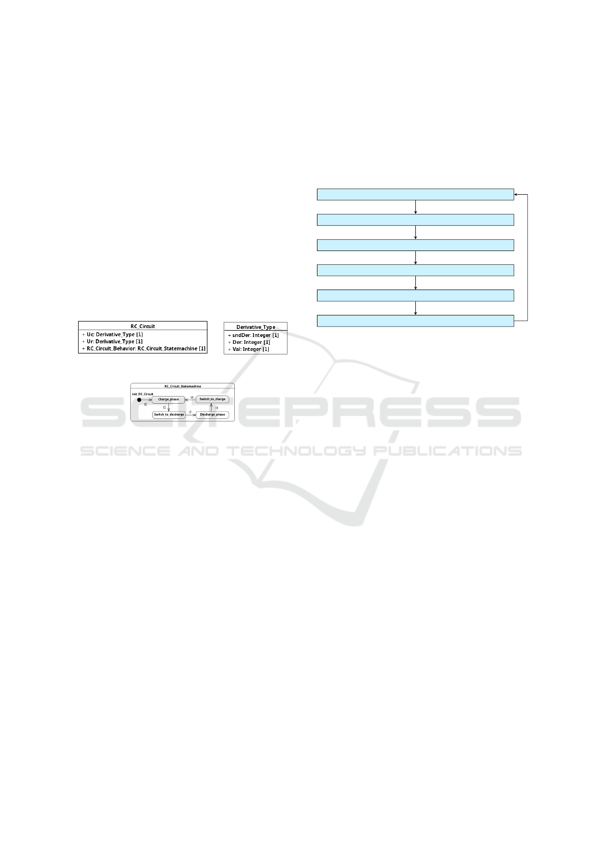
SysML RC Circuit Block. The RC circuit is mod-
eled in a SysML block as shown in Figure 12. It has 3
attributes, the first two are the variables of the system:
U
c
and U
r
. Their type is Derivative_Type which rep-
resents a value and its first and second derivative. The
last attribute is typed as a state machine that specifies
the behavior of the RC circuit.
Figure 12: Block Definition Diagram of the RC circuit.
Figure 13: State Machine Diagram of the RC circuit.
RC Circuit State Machine. The equations of the
RC circuit are modeled by a state machine with 5
states and 5 transitions as shown in Figure 13:
• the t
0
transition sets the initial values of the states
variables U
c
to = 0 and U
r
to > 0, and sets the first
derivative of U
c
to > 0 and U
r
to < 0;
• t
1
flips the switch to the discharge position, and
sets the first derivative of U
r
to < 0 and U
c
to < 0;
• t
2
flips the switch to the discharge position, and
sets the first derivative of U
r
to > 0 and U
c
to < 0;
• t
3
flips the switch to the charging position, and
sets the first derivative of U
r
to > 0 and U
c
to > 0;
• t
4
flips the switch back to charging, and sets the
first derivative of U
c
to > 0 and U
r
to < 0.
Our QVT operational transformation turns this
SysML model into a HyDiv model.
Diversity Model of the RC Circuit. Then our Ac-
celeo transformation produces the Xlia source code
of the Diversity model of the system from this Hy-
Div model. This transformation encodes the seman-
tics of our model of execution. It generates the au-
tomaton for the system, as well as the automata for
the state variables and their derivatives, and the au-
tomaton which computes the qualitative variation of
these variables.
Qualitative Behavior Computed by Diversity.
Running Diversity on the Xlia model, we obtain the
qualitative behavior shown in Figure 14.
Charge_phase, Decrease_Ur, Increase_Uc
Switch_to_discharge, Decrease_Ur, Angular_Decrease_Uc
Discharge_phase, Angular_Increase_Ur, Decrease_Uc
Discharge_phase, Increase_Ur, Decrease_Uc
Switch_to_charge, Increase_Ur, Angular_Increase_Uc
Charge_phase, Angular_Decrease_Ur, Increase_Uc
Figure 14: Qualitative behavior of the RC circuit.
We see clearly in this figure that the voltage U
r
across resistor R and the voltage U
c
across capacitor
C are varying in opposite ways:
• in the Charge_phase, U
r
is in a Decreasing_state
while U
c
is in an Increasing_state;
• in the Switch_to_discharge, U
r
is still in a De-
creasing_state because it must go to −E while
U
c
is in an Angular_Decreasing_state because the
capacitor starts discharging;
• in the Discharge_phase, U
r
is in an Increas-
ing_state while U
c
is in a Decreasing_state;
• in the Switch_to_charge, U
r
is still in an Increas-
ing_state because it must go to +E while U
c
is in
an Angular_Increasing_state because the capaci-
tor starts charging.
4 DISCUSSION
The qualitative simulation of the bouncing ball pro-
duces other behaviors than the one presented here.
In our previous work in (Medimegh et al., 2016),
we described two behaviors that were impossible and
should be eliminated. Thanks to our new model of
execution, which computes qualitative variations of
the first derivative such as Increasingly_Increase, we
were able to eliminate them. For instance, when the
ball is falling, its speed is negative and decreasing
(because the second derivative is negative). The new
model of execution identifies the qualitative variation
of the height of the ball as Increasingly_Decrease.
Qualitative Simulation of Hybrid Systems with an Application to SysML Models
285

Starting from a positive symbolic value, the height of
the ball has to become null at some point, which elim-
inates the behavior where the ball was falling forever
toward the ground without ever reaching it.
Some behaviors found by Diversity differ only by
a few sequences of states. This is due to the way
Diversity detects Redundancy. During the symbolic
execution of a model, Diversity builds a tree, each
branch corresponding to a choice for the symbolic
value of the variables. When it finds an execution con-
text that was met before, it cuts the execution of this
branch, and makes it point to the state that was met
before. This turns the tree into an execution graph,
and makes it possible to capture infinite behaviors in
a finite structure. However, depending on the order in
which the variables change, the redundancy detection
can be delayed, which creates several execution paths
for the same physical behavior. We plan to filter the
results of Diversity in order to keep only one path for
each possible physical behavior of the hybrid system.
5 CONCLUSION
We have presented a new symbolic execution model
for the qualitative simulation of hybrid systems us-
ing only a qualitative model of the equations, with
a symbolic integration of the derivatives of the state
variables. This execution model is implemented us-
ing state machines, which are executed symbolically
by the Diversity tool, yielding the possible qualitative
behaviors of the system.
Compared to our previous work (Medimegh et al.,
2016), symbolic integration allows for determinis-
tic automata and a reduced set of qualitative behav-
iors. Computing higher order qualitative states also
allowed us to eliminate impossible behaviors by for-
bidding some transitions. This execution model there-
fore provides a better abstraction of the behavior of
the system. The example of the RC circuit shows that
this model can be adapted to first order models.
We apply this approach to the analysis of SysML
models, using an M2M transformation from SysML
to a pivot language, and an M2T transformation from
this language to Diversity, allowing the tool chain to
be adapted to other input and output languages.
We plan to enrich the symbolic execution model
with a filter to eliminate redundant symbolic behav-
iors that correspond to the same physical behavior in
the execution tree generated by Diversity. Another
track to explore is to design a SysML profile for qual-
itative simulation without differential equations, in or-
der to make the qualitative modeling of hybrid system
in SysML easier and more expressive.
There are obviously limitations to the analysis
of hybrid systems using qualitative simulation with-
out differential equations, because behaviors that de-
pend on specific numerical values of some parame-
ters cannot be identified. However, this approach can
be applied to systems that cannot be analyzed more
precisely because their differential equations are too
complex. It can also be applied in the early phases of
the design of a system, when some parameters or the
exact differential equations are not known yet.
REFERENCES
Berleant, D. and Kuipers, B. (1992). Qualitative-numeric
simulation with q3. Recent advances in qualitative
physics, 98:285–313.
Bredeweg, B., Linnebank, F., Bouwer, A., and Liem, J.
(2009). Garp3—workbench for qualitative modelling
and simulation. Ecological informatics, 4(5):263–
281.
Brown, C. W. (2003). Qepcad b: A program for computing
with semi-algebraic sets using cads. SIGSAM Bull.,
37(4):97–108.
de Kleer, J. and Bobrow, D. G. (1984). Qualitative rea-
soning with higher-order derivatives. In AAAI, pages
86–91.
Fouché, P. and Kuipers, B. J. (1992). Reasoning about en-
ergy in qualitative simulation. IEEE Trans. on Sys-
tems, Man, and Cybernetics, 22(1):47–63.
Gallois, J.-P. and Pierron, J.-Y. (2016). Qualitative simu-
lation and validation of complex hybrid systems. In
ERTS 2016, TOULOUSE, France.
Kuipers, B. (1986). Qualitative simulation. Artificial intel-
ligence, 29(3):289–338.
Kuipers, B. and Chiu, C. (1987). Taming intractible branch-
ing in qualitative simulation. Readings in qualitative
reasoning about physical systems.
Lynch, N., Segala, R., and Vaandrager, F. (2003). Hybrid i/o
automata. Information and computation, 185(1):105–
157.
Medimegh, S., Pierron, J.-Y., Gallois, J.-P., and Boulanger,
F. (2016). A new approach of qualitative simulation
for the validation of hybrid systems. In GEMOC at
MODELS 2016.
Missier, A. and Trave-Massuyes, L. (1991). Temporal in-
formation in qualitative simulation. In AI, Simulation
and Planning in High Autonomy Systems, pages 298–
305. IEEE.
Rapin, N., Gaston, C., Lapitre, A., and Gallois, J.-P. (2003).
Behavioural unfolding of formal specifications based
on communicating automata. In Proc. 1st Workshop
on Automated Technology for Verification and Analy-
sis.
Shen, Q. and Leitch, R. (1990). Integrating common-sense
and qualitative simulation by the use of fuzzy sets.
In 4th International Workshop on Qualitative Physics,
pages 220–232.
MODELSWARD 2018 - 6th International Conference on Model-Driven Engineering and Software Development
286
