Parameter Learning for Spiking Neural Networks

Modelled as Timed Automata

Elisabetta De Maria and Cinzia Di Giusto

Universit

e C

ote d’Azur, CNRS, I3S, France

Keywords:

Neural Networks, Parameter Learning, Timed Automata, Temporal Logic, Model Checking.

Abstract:

In this paper we present a novel approach to automatically infer parameters of spiking neural networks. Neu-

rons are modelled as timed automata waiting for inputs on a number of different channels (synapses), for

a given amount of time (the accumulation period). When this period is over, the current potential value is

computed considering current and past inputs. If this potential overcomes a given threshold, the automaton

emits a broadcast signal over its output channel, otherwise it restarts another accumulation period. After each

emission, the automaton remains inactive for a ﬁxed refractory period. Spiking neural networks are formalised

as sets of automata, one for each neuron, running in parallel and sharing channels according to the network

structure. This encoding is exploited to ﬁnd an assignment for the synaptical weights of neural networks such

that they can reproduce a given behaviour. The core of this approach consists in identifying some correcting

actions adjusting synaptical weights and back-propagating them until the expected behaviour is displayed. A

concrete case study is discussed.

1 INTRODUCTION

The brain behaviour is the object of thorough studies:

researchers are interested not only in the inner func-

tioning of neurons (which are its elementary compo-

nents), their interactions and the way these aspects

participate to the ability to move, learn or remember,

typical of living beings; but also in reproducing such

capabilities (emulating nature), e.g., within robot con-

trollers, speech/text/face recognition applications, etc.

In order to achieve a detailed understanding of the

brain functioning, both neurons behaviour and their

interactions must be studied. Several models of the

neuron behaviour have been proposed: some of them

make neurons behave as binary threshold gates, other

ones exploit a sigmoidal transfer function, while, in

many cases, differential equations are employed. Ac-

cording to (Paugam-Moisy and Bohte, 2012; Maass,

1997), three different and progressive generations of

neural networks can be recognised: (i) ﬁrst genera-

tion models handle discrete inputs and outputs and

their computational units are threshold-based transfer

functions; they include McCulloch and Pitt’s thresh-

old gate model (McCulloch and Pitts, 1943), the per-

ceptron model(Freund and Schapire, 1999), Hopﬁeld

networks (Hopﬁeld, 1988), and Boltzmann machines

(Ackley et al., 1988); (ii) second generation models

exploit real valued activation functions, e.g., the sig-

moid function, accepting and producing real values:

a well known example is the multi-layer perceptron

(Cybenko, 1989; Rumelhart et al., 1988); (iii) third

generation networks are known as spiking neural net-

works. They extend second generation models treat-

ing time-dependent and real valued signals often com-

posed by spike trains. Neurons may ﬁre output spikes

according to threshold-based rules which take into ac-

count input spike magnitudes and occurrence times

(Paugam-Moisy and Bohte, 2012).

The core of our analysis are spiking neural net-

works (Gerstner and Kistler, 2002). Because of the

introduction of timing aspects they are considered

closer to the actual brain functioning than other gen-

erations models. Spiking neurons emit spikes taking

into account input impulses strength and their occur-

rence instants. Models of this sort are of great inter-

est, not only because they are closer to natural neural

networks behaviour, but also because the temporal di-

mension allows to represent information according to

various coding schemes (Recce, 1999; Paugam-Moisy

and Bohte, 2012): e.g., the amount of spikes occurred

within a given time window (rate coding), the recep-

tion/absence of spikes over different synapses (binary

coding), the relative order of spikes occurrences (rate

rank coding), or the precise time difference between

any two successive spikes (timing coding). Several

spiking neuron models have been proposed in the lit-

Maria, E. and Giusto, C.

Parameter Learning for Spiking Neural Networks Modelled as Timed Automata.

DOI: 10.5220/0006530300170028

In Proceedings of the 11th International Joint Conference on Biomedical Engineering Systems and Technologies (BIOSTEC 2018) - Volume 3: BIOINFORMATICS, pages 17-28

ISBN: 978-989-758-280-6

erature, having different complexities and capabili-

ties. Our aim is to produce a neuron model be-

ing meaningful from a biological point of view but

also amenable to formal analysis and veriﬁcation, that

could be therefore used to detect non-active portions

within some network (i.e., the subset of neurons not

contributing to the network outcome), to test whether

a particular output sequence can be produced or not,

to prove that a network may never be able to emit, to

assess if a change to the network structure can alter its

behaviour, or to investigate (new) learning algorithms

which take time into account.

In this paper we focus on the leaky integrate &

ﬁre (LI&F) model originally proposed in (Lapicque,

1907). It is a computationally efﬁcient approximation

of single-compartment model (Izhikevich, 2004) and

is abstracted enough to be able to apply formal veri-

ﬁcation techniques such as model-checking. Here we

work on an extended version of the discretised formu-

lation proposed in (De Maria et al., 2016), which re-

lies on the notion of logical time. Time is considered

as a sequence of logical discrete instants, and an in-

stant is a point in time where external input events can

be observed, computations can be done, and outputs

can be emitted. The variant we introduce here takes

into account some new time-related aspects, such as a

lapse of time in which the neuron is not active, i.e., it

cannot receive and emit. We encode LI&F networks

into timed automata: we show how to deﬁne the be-

haviour of a single neuron and how to build a network

of neurons. Timed automata (Alur and Dill, 1994) are

ﬁnite state automata extended with timed behaviours:

constraints are allowed to limit the amount of time

an automaton can remain within a particular state, or

the time interval during which a particular transition

may be enabled. Timed automata networks are sets of

automata that can synchronise over channel commu-

nications.

Our modelling of spiking neural networks consists

of timed automata networks where each neuron is an

automaton. Its behaviour consists in accumulating the

weighted sum of inputs, provided by a number of in-

going weighted synapses, for a given amount of time.

Then, if the potential accumulated during the last

and previous accumulation periods overcomes a given

threshold, the neuron ﬁres an output over the outgo-

ing synapse. Synapses are channels shared between

the timed automata representing neurons, while spike

emissions are represented by broadcast synchronisa-

tions occurring over such channels. Timed automata

are also exploited to produce or recognise precisely

deﬁned spike sequences.

The closest related work is (Aman and Ciobanu,

2016). The authors provide a mapping of spiking neu-

ral P systems into timed automata. The underlying

model is considerably different from ours: refractory

period is considered in terms of number of applica-

tion of rules instead of durations and inhibitions are

represented as forgetting rules while we use negative

weights. Unlike our approach, where the dynamics is

compositional and implicit in the structure of the net-

work, in (Aman and Ciobanu, 2016) the semantics is

the result of the encoding of rules and neurons.

As a main contribution, we exploit our automata-

based modelling to propose a new methodology for

parameter inference in spiking neural networks. In

particular, our approach allows to ﬁnd an assignment

for the synaptical weights of a given neural network

such that it can reproduce a given behaviour. We bor-

row inspiration from the SpikeProp rule (Bohte et al.,

2002), a variant of the well known back-propagation

algorithm (Rumelhart et al., 1988) used for supervised

learning in second generation learning. The Spike-

Prop rule deals with multi-layered cycle-free spiking

neural networks and aims at training networks to pro-

duce a given output sequence for each class of input

sequences. The main difference with respect to our

approach is that we are considering here a discrete

model and our networks are not multi-layered. We

also rest on Hebb’s learning rule (Hebb, 1949) and

its time-dependent generalisation rule, the spike tim-

ing dependent plasticity (STDP) rule (Sj

ostr

om and

Gerstner, 2010): they both act locally, with respect to

each neuron, i.e., no prior assumption on the network

topology is required in order to compute the weight

variations for some neuron input synapses. Differ-

ently from STDP, our approach takes into account

not only recent spikes but also some external feed-

back (advices) in order to determine which weights

should be modiﬁed and whether they must increase

or decrease. Moreover, we do not prevent excitatory

synapses from becoming inhibitory (or vice versa),

which is usually a constraint for STDP implementa-

tions. A general overview on spiking neural network

learning approaches and open problems in this con-

text can be found in (Gr

uning and Bohte, 2014).

We apply the proposed approach to ﬁnd suitable

parameters in mutual inhibition networks, a well stud-

ied class of networks in which the constituent neurons

inhibit each other neuron’s activity (Matsuoka, 1987).

The rest of the paper is organised as follows: in

Section 2 we describe our reference model, the leaky

integrate & ﬁre one, in Section 3 we recall deﬁnitions

of timed automata networks and temporal logics, and

in Section 4 we show how spiking neural networks

can be encoded into timed automata networks and

how inputs and outputs are handled by automata. In

Section 5 we develop the novel parameter learning ap-

BIOINFORMATICS 2018 - 9th International Conference on Bioinformatics Models, Methods and Algorithms

proach and we introduce a case study. Finally, Section

6 summarises our contribution and presents some fu-

ture research directions. An Appendix with additional

material is added for the reader convenience.

2 LEAKY INTEGRATE AND FIRE

MODEL

Spiking neural networks (Maass, 1997) are modelled

as directed weighted graphs where vertices are com-

putational units and edges represent synapses. The

signals propagating over synapses are trains of im-

pulses: spikes. Synapses may modulate these signals

according to their weight: excitatory if positive, or in-

hibitory if negative.

The dynamics of neurons is governed by their

membrane potential (or, simply, potential), represent-

ing the difference of electrical potential across the

cell membrane. The membrane potential of each neu-

ron depends on the spikes received over the ingoing

synapses. Both current and past spikes are taken into

account, even if old spikes contribution is lower. In

particular, the leak factor is a measure of the neu-

ron memory about past spikes. The neuron outcome

is controlled by the algebraic difference between its

membrane potential and its ﬁring threshold: it is en-

abled to ﬁre (i.e., emit an output impulse over all

outgoing synapses) only if such a difference is non-

negative. Spike propagation is assumed to be instan-

taneous. Immediately after each emission the neuron

membrane potential is reset and the neuron stays in a

refractory period for a given amount of time. During

this period it has no dynamics: it cannot increase its

potential as any received spike is lost and therefore it

cannot emit any spike.

Deﬁnition 1 (Spiking Integrate and Fire Neural Net-

work). A spiking integrate and ﬁre neural network is

a tuple (V, A, w), where:

• V are spiking integrate and ﬁre neurons,

• A ⊆ V ×V are synapses,

• w : A → Q ∩[−1,1] is the synapse weight function

associating to each synapse (u, v) a weight w

u,v

We distinguish three disjoint sets of neurons: V

(input

neurons), V

int

(intermediary neurons), and V

(output

neurons), with V = V

∪V

int

∪V

A spiking integrate and ﬁre neuron v is characterized

by a parameter tuple (θ

,τ

,λ

, p

), where:

• θ

∈ N is the ﬁring threshold,

• τ

∈ N

is the refractory period,

• λ

∈ Q ∩ [0, 1] is the leak factor.

The dynamics of a spiking integrate and ﬁre neuron v

is given by:

• p

: N → Q

is the [membrane] potential function

deﬁned as

(t) =



∑

i=1

· x

(t), if p

(t − 1) > θ

∑

i=1

· x

(t)+ λ

· p

(t − 1), o/w.

with p

(0) = 0 and where x

(t) ∈ {0,1} is the sig-

nal received at the time t by the neuron through its

out of m input synapses (observe that the past

potential is multiplied by the leak factor while cur-

rent inputs are not weakened),

• y

: N → {0,1} is the neuron output function, de-

ﬁned as

(t) =

(

1 if p

(t) > θ

0 otherwise.

As shown in the previous deﬁnition, the set of neu-

rons of a spiking integrate and ﬁre neural network can

be classiﬁed into input, intermediary, and output ones.

Each input neuron can only receive as input external

signals (and not other neurons’ output). The output

of each output neuron is considered as an output for

the network. Output neurons are the only ones whose

output is not connected to other neurons.

3 PRELIMINARIES: TIMED

AUTOMATA AND TEMPORAL

LOGIC

This section is devoted to the introduction of the for-

mal tools we adopt in the rest of the paper, namely

timed automata and temporal logics.

Timed Automata. Timed automata (Alur and Dill,

1994) are a powerful theoretical formalism for mod-

elling and verifying real time systems. A timed

automaton is an annotated directed (and connected)

graph, with an initial node and provided with a ﬁ-

nite set of non-negative real variables called clocks.

Nodes (called locations) are annotated with invariants

(predicates allowing to enter or stay in a location),

arcs with guards, communication labels, and possi-

bly with some variables upgrades and clock resets.

Guards are conjunctions of elementary predicates of

the form x op c, where op ∈ {>, ≥,=,<, ≤}, x is a

clock, and c a (possibly parameterised) positive inte-

ger constant. As usual, the empty conjunction is in-

terpreted as true. The set of all guards and invariant

predicates will be denoted by G.

Parameter Learning for Spiking Neural Networks Modelled as Timed Automata

Deﬁnition 2. A timed automaton TA is a tuple

(L,l

,X,Var, Σ,Arcs,Inv), where

• L is a set of locations with l

∈ L the initial one

• X is the set of clocks,

• Var is a set of integer variables,

• Σ is a set of communication labels,

• Arcs ⊆ L × (G ∪ Σ ∪ U) × L is a set of arcs be-

tween locations with a guard in G, a communica-

tion label in Σ ∪ {ε}, and a set of variable (linear

arithmetics) upgrades and clock resets;

• Inv : L → G assigns invariants to locations.

It is possible to deﬁne a synchronised product of

a set of timed automata that work and synchronise in

parallel. The automata are required to have disjoint

sets of locations, but may share clocks and communi-

cation labels which are used for synchronisation. We

restrict communications to be broadcast through la-

bels b!,b? ∈ Σ, meaning that a set of automata can

synchronise if one is emitting; notice that a process

can always emit (e.g., b!) and the receivers (b?) must

synchronise if they can.

Locations can be normal, urgent or committed.

Urgent locations force the time to freeze, committed

ones freeze time and the automaton must leave the

location as soon as possible, i.e., they have higher pri-

ority.

The synchronous product TA

k ... k TA

timed automata, where for each j ∈ [1,. .., n], TA

,Var

,Arcs

,Inv

) and all L

are pairwise

disjoint sets of locations, is the timed automaton

TA = (L,l

,X,Var, Σ,Arcs,Inv)

such that:

• L = L

× .. . × L

and l

= (l

,.. .,l

• X =

j=1

• Var =

j=1

Var

• Σ =

j=1

• Arcs is the set of arcs (l

,.. .,l

)

g,a,u

−→ (l

,.. .,l

)

such that for all 1 ≤ j ≤ n then l

= l

• ∀l = (l

,.. .,l

) ∈ L : Inv(l) =

Inv

The semantics of a synchronous product TA

... k TA

is the one of the underlying timed automaton

TA with the following notations. A location is a vec-

tor l = (l

,.. .,l

). We write l[l

, j ∈ S] to denote

the location l in which the j

element l

is replaced

by l

, for all j in some set S. A valuation is a func-

tion ν from the set of clocks to the non-negative reals.

Let V be the set of all clock valuations, and ν

(x) = 0

for all x ∈ X. We shall denote by ν  F the fact that

the valuation ν satisﬁes (makes true) the formula F.

If r ∈ U is a clock reset, we shall denote by ν[r] the

valuation obtained after applying the clock reset to ν;

and if d ∈ R

is a delay, ν + d is the valuation such

that, for any clock x ∈ X, (ν + d)(x) = ν(x) + d. Fi-

nally, we use f to denote a valuation of variables in

Var, the set of all valuations is denoted F , f

(v) = 0

for all v ∈ Var and f [u] is the application of upgrades

in u to variables in Var.

The semantics of a synchronous product TA

... k TA

is deﬁned as a timed transition system

(S,s

,→), where S = (L

×,.. . × L

) × V × F is the

set of states, s

= (l

,ν

, f

) is the initial state, and

→⊆ S × S is the transition relation deﬁned by:

• (silent): (l, ν, f ) → (l

,ν

, f [u]) if there exists

g,ε,u

−→ l

, for some i, such that l

= l[l

], ν  g

and ν

= ν[r],

• (broadcast): (

l,ν, f ) → (

,ν

, f [u]) if there exists

an output arc l

,b!,u

−→ l

∈ Arcs

and a (possi-

bly empty) set of input arcs of the form l

,b?,u

−→

∈ Arcs

such that for all k ∈ K = {k

,.. .,k

} ⊆

,.. .,l

} \ {l

}, the size of K is maximal, ν 

k∈K∪{ j}

, l

= l[l

,k ∈ K ∪ { j}] and ν

ν[r

,k ∈ K ∪ { j}];

• (timed): (l,ν, f ) → (l, ν + d, f ) if ν + d  Inv(l).

The valuation function ν is extended to handle a

set of shared bounded integer variables: predicates

concerning such variables can be part of edges guards

or locations invariants, moreover variables can be up-

dated on edges ﬁrings but they cannot be assigned to

or from clocks.

In Appendix A we exemplify timed automata us-

age. Throughout our modelling, we have used the

speciﬁcation and analysis tool Uppaal (Bengtsson

et al., 1995), which provides the possibility of design-

ing and simulating timed automata networks on top of

the ability of testing networks against temporal logic

formulae.

Temporal Logics and Model Checking. Model

checking is one of the most common approaches to

the veriﬁcation of software and hardware (distributed)

systems (Clarke et al., 1999). It allows to automati-

cally prove whether a system veriﬁes or not a given

speciﬁcation. In order to apply such a technique, the

system at issue should be encoded as a ﬁnite transi-

tion system and the speciﬁcation should be written

using propositional temporal logic. Formally, a tran-

sition system over a set AP of atomic propositions

is a tuple M = (Q, T,L), where Q is a ﬁnite set of

states, T ⊆ Q × Q is a total transition relation, and

L : Q → 2

is a labelling function that maps every

BIOINFORMATICS 2018 - 9th International Conference on Bioinformatics Models, Methods and Algorithms

state into the set of atomic propositions that hold at

that state.

Temporal logics are formalisms for describing

the dynamical evolution of a given system (Hughes

and Cresswell, 1968). The computation tree logic

CTL

∗

allows to describe properties of computation

trees. Its formulas are obtained by (repeatedly) apply-

ing Boolean connectives, path quantiﬁers, and state

quantiﬁers to atomic formulas. The path quantiﬁer

A (resp., E) can be used to state that all the paths

(resp., some path) starting from a given state have

some property. The state quantiﬁers are X (next time),

which speciﬁes that a property holds at the next state

of a path, F (sometimes in the future), which requires

a property to hold at some state on the path, G (always

in the future), which imposes that a property is true at

every state on the path, and U (until), which holds if

there is a state on the path where the second of its ar-

gument properties holds and, at every preceding state

on the path, the ﬁrst of its two argument properties

holds.

The branching time logic CTL is a fragment of

CTL

∗

that allows quantiﬁcation over the paths starting

from a given state. Unlike CTL

∗

, it constrains every

state quantiﬁer to be immediately preceded by a path

quantiﬁer.

Given a transition system M = (Q,T, L), a state

q ∈ Q, and a temporal logic formula ϕ expressing

some desirable property of the system, the model

checking problem consists of establishing whether ϕ

holds at q or not, namely, whether M,q |= ϕ.

4 SPIKING NEURAL NETWORKS

MODELLING

We present here our modelling of spiking integrate

and ﬁre neural networks (in the following denoted as

neural networks) via timed automata networks. Let

S = (V,A, w) be a neural network, G be a set of input

generator neurons (these ﬁctitious neurons are con-

nected to input neurons and generate input sequences

for the network), and O be a set of output consumer

neurons (these ﬁctitious neurons are connected to the

broadcast channel of each output neuron and aim at

consuming their emitted spikes). The correspond-

ing timed automata network is obtained as the syn-

chronous product of the encoding of input generator

neurons, the neurons of the network (referred as stan-

dard neurons in the following), and output consumers

neurons. More formally:

JSK = ( k

∈G

K) k ( k

∈V

K) k ( k

∈O

Input Generators. The behaviour of input genera-

tor neurons is part of the speciﬁcation of the network.

Here we deﬁne two kinds of input behaviours: regu-

lar and non-deterministic ones. For each family, we

provide an encoding into timed automata.

Regular Input Sequences. Spike trains are “regu-

lar” sequences of spikes and pauses: spikes are instan-

taneous while pauses have a non-null duration. Se-

quences can be empty, ﬁnite or inﬁnite. After each

spike there must be a pause, except when the spike is

the last event of a ﬁnite sequence. Inﬁnite sequences

are composed by two parts: a ﬁnite and arbitrary pre-

ﬁx and an inﬁnite and periodic part composed by a ﬁ-

nite sequence of spike–pause pairs which is repeated

inﬁnitely often. More formally, such sequences are

given in terms of the following grammar:

B ::= Φ.(Φ)

| P(d).Φ.(Φ)

Φ ::= s.P(d).Φ | ε

with s representing a spike and P(d) a pause of dura-

tion d. The automaton generating input sequences is

given in Appendix B.1.

Non-deterministic Input Sequences. This kind of

input sequences is useful when no assumption is

available on neuron inputs. These are random se-

quences of spikes separated by at least T

min

time units.

Their precise encoding is given in Appendix B.2.

Standard Neurons. The neuron is a computational

unit behaving as follows: i) it accumulates potential

whenever it receives input spikes within a given ac-

cumulation period, ii) if the accumulated potential is

greater than the threshold, it emits an output spike, iii)

it waits during a refractory period, and restarts from

i). Observe that the accumulation period is not present

in the deﬁnition of neuron (Def. 1). It is indeed intro-

duced here to slice time and therefore discretise the

decrease of the potential value due to the leak factor.

We assume that two input spikes on the same synapse

cannot be received within the same accumulation pe-

riod (i.e., the accumulation period is shorter than the

minimum refractory period of the input neurons of the

network). Next, we give the encoding of neurons into

timed automata.

Deﬁnition 3. Given a neuron v = (θ,τ,λ, p,y) with

m input synapses, its encoding into timed automata is

N = (L, A,X,Var, Σ,Arcs,Inv) with:

• L = {A,W,D} with D committed,

• X = {t}

• Var = {p,a}

Parameter Learning for Spiking Neural Networks Modelled as Timed Automata

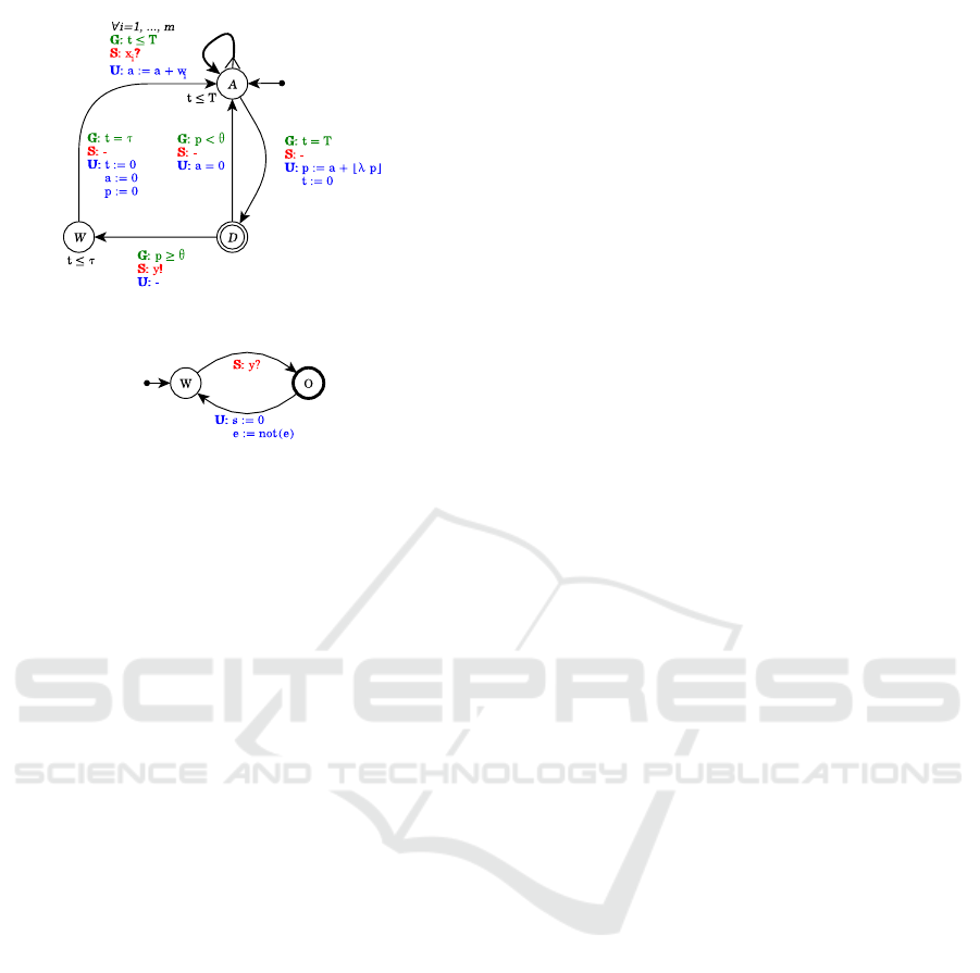
(a) Neuron model.

(b) Output consumer au-

tomaton.

Figure 1: Automata for standard neuron and output con-

sumer.

• Σ = {x

| i ∈ [1..m]} ∪ {y},

• Arcs = {(A,t ≤ T, x

?,{a := a + w

},A) |

i ∈ [1..m]} ∪ {(A,t = T, ,{p := a +

bλpc}, D),(D, p < θ, ,{a := 0},A), (D, p ≥

θ,y!, ,W),(W,t = τ, ,{a := 0,t := 0, p :=

0},A)} ;

• Inv(A) = t ≤ T, Inv(W) = t ≤ τ,Inv(D) = true.

The neuron behaviour, described by the automa-

ton in Figure 1(a), depends on the following channels,

variables and clocks:

• x

for i ∈ [1..m] are the m input channels,

• y is the broadcast channel used to emit the output

spike,

• p ∈ N is the current potential value, initially set to

zero,

• a ∈ N is the weighted sum of input spikes occurred

within the current accumulation period; it equals

zero at the beginning of each round.

The behaviour of the automaton modelling neuron

v can be summed up as follows:

• the neuron keeps waiting in state A (for Accumu-

lation) for input spikes while t 6 T and, whenever

it receives a spike on input x

, it updates a with

a := a + w

;

• when t = T , the neuron moves to state D (for De-

cision), resetting t and updating p according to the

potential function given in Deﬁnition 1:

p := a +

λ · p

Since state D is committed, it does not allow time

to progress, so, from this state, the neuron can

move back to state A resetting a if the potential

has not reached the threshold p < θ, or it can move

to state W, ﬁring an output spike, otherwise;

• the neuron remains in state W (for Wait) for τ time

units (τ is the length of the refractory period) and

then it moves back to state A resetting a, p and t.

Output Consumers. In order to have a complete

modelling of a spiking neural network, for each out-

put neuron we build an output consumer automa-

ton O

. The automaton, whose formal deﬁnition is

straightforward, is shown in Figure 1(b). The con-

sumer waits in location W for the corresponding out-

put spikes on channel y and, as soon as it receives the

spike, it moves to location O. This location is only

needed to simplify model checking queries. Since it

is urgent, the consumer instantly moves back to loca-

tion W resetting s, the clock measuring the elapsed

time since last emission, and setting e to its negation,

with e being a boolean variable which differentiates

each emission from its successor.

We have a complete implementation of the spiking

neural network model proposed in the paper via the

tool Uppaal. It can be found on the web page (Ciatto

et al., ). We have validated our neuron model against

some characteristic properties studied in (Izhikevich,

2004) (tonic spiking, excitability, integrator, etc.).

These properties have been formalised in temporal

logics and checked via model-checking tools. All ex-

periments and results can be found in (Ciatto et al.,

2017).

Observe that, since we rely on a discrete time, we

could have used tick automata (Gruber et al., 2005), a

variant of B

uchi automata where a special clock mod-

els the discrete ﬂow of time. However, to the best of

our knowledge, no existing tool allows to implement

such automata. We decided to opt for timed automata

in order to have an effective implementation of our

networks to be exploited in parameter learning algo-

rithms.

5 PARAMETER INFERENCE

In this section we examine the Learning Problem: i.e.,

how to determine a parameter assignment for a net-

work with a ﬁxed topology and a given input such

that a desired output behaviour is displayed. Here we

only focus on the estimation of synaptic weights in

a given spiking neural network; the generalisation of

our methodology to other parameters is left for future

work.

BIOINFORMATICS 2018 - 9th International Conference on Bioinformatics Models, Methods and Algorithms

Our analysis takes inspiration from the SpikeProp

algorithm (Bohte et al., 2002); in a similar way, here,

the learning process is led by supervisors. Differ-

ently from the previous section, each output neuron

is linked to a supervisor instead of an output con-

sumer. Supervisors compare the expected output be-

haviour with the one of the output neuron they are

connected to. Thus either the output neuron behaved

consistently or not. In the second case and in order to

instruct the network, the supervisor back-propagates

advices to the output neuron depending on two pos-

sible scenarios: i) the neuron ﬁres a spike, but it was

supposed to be quiescent, ii) the neuron remains qui-

escent, but it was supposed to ﬁre a spike. In the

ﬁrst case the supervisor addresses a should not have

ﬁred message (SNHF) and in the second one a should

have ﬁred (SHF). Then each output neuron modiﬁes

its ingoing synaptic weights and in turn behaves as

a supervisor with respect to its predecessors, back-

propagating the proper advice.

The advice back-propagation (ABP) algorithm ba-

sically lies on a depth-ﬁrst visit of the graph topology

of the network. Let N

be the i-th predecessor of an

automaton N , then we say that N

ﬁred recently, with

respect to N , if N

ﬁred during the current or pre-

vious accumulate-ﬁre-wait cycle of N . Thus, upon

reception of a SHF message, N has to strengthen

the weight of each ingoing excitatory synapse corre-

sponding to a neuron which ﬁred recently and weaken

the weight of each ingoing inhibitory synapse cor-

responding to a neuron which did not ﬁre recently.

Then, it propagates a SHF advice to each ingoing ex-

citatory synapse corresponding to a neuron which did

not ﬁre recently, and symmetrically a SNHF advice

to each ingoing inhibitory synapse corresponding to

a neuron which ﬁred recently (see Algorithm 1 for

SHF, Algorithm 2 for the dual case of SNHF in given

in Appendix C; in both algorithms, ∆ is a constant

factor used to manage increments).

When the graph visit reaches an input generator, it

will simply ignore any received advice (because input

sequences should not be affected by the learning pro-

cess). The learning process ends when all supervisors

do not detect any more errors.

Example 1 (Turning on and off a diamond structure

of neurons.). This example shows how the ABP al-

gorithm can be used to make a neuron emit at least

once in a spiking neural network having the diamond

structure shown in Figure 2. We assume that N

fed by an input generator I that continuously emits

spikes. No neuron in the network is able to emit be-

cause all the weights of their input synapses are equal

to zero and their thresholds are higher than zero. We

want the network to learn a weight assignment so that

Algorithm 1 : Abstract ABP: Should Have Fired advice

pseudo-code.

1: procedure SHOULD-HAVE-FIRED(neuron)

2: if IS-VISITED(neuron) then

3: return

4: SET-VISITED(neuron, True)

5: for i ← 1 ... COUNT-

PREDECESSORS(neuron) do

6: weight

← GET-WEIGHT(neuron, i)

7: f ired

← FIRED-RECENTLY(neuron, i)

8: neuron

← GET-PREDECESSOR(neuron,

9: INCREASE-WEIGHT(neuron, i, ∆)

10: if weight

≥ 0 then

11: if ¬ f ired

then

12: SHOULD-HAVE-FIRED(neuron

)

13: else

14: if f ired

then

15: SHOULD-NOT-HAVE-

FIRED(neuron

)

I,1

1,2

1,3

3,4

2,4

Figure 2: A neural network with a diamond structure.

is able to emit, that is, to produce a spike after an

initial pause.

At the beginning we expect no activity from neu-

ron N

. As soon as the initial pause is elapsed, we

require a spike but, as all weights are equal to zero,

no emission can happen. Thus a SHF advice is back-

propagated to neurons N

and N

and consequently

to N

. The process is then repeated until all weights

stabilise and neuron N

is able to ﬁre.

There are several possibilities on how to realise

supervisors and the ABP algorithm. The approach we

choose is a model checking oriented one, where su-

pervisors are represented by temporal logic formulae.

Model-checking-oriented Advice Back-

Propagation. In the following we propose a

model checking-driven approach to parameter

learning. Such a technique consists in iterating

the learning process until a desired CTL property

concerning the output of the network is veriﬁed.

Parameter Learning for Spiking Neural Networks Modelled as Timed Automata

The hypothesis we introduce are the following

ones: (i) input generators, standard neurons, and out-

put consumers share a global clock which is never re-

set and (ii) for each output consumer, there exists a

clock measuring the elapsed time since the last re-

ceived spike. The CTL formula specifying the ex-

pected output of the network can only contain pred-

icates relative to the output consumers and the global

clock. At each step of the algorithm, we make an ex-

ternal call to the model checker to test whether the

network satisﬁes the formula or not. If the formula

is veriﬁed, the learning process ends; otherwise, the

model checker provides a trace as a counterexample.

Such a trace is exploited to derive the proper correc-

tive action to be applied to each output neuron, that

is, the invocation of either the SHF procedure, or the

SNHF procedure previously described (or no proce-

dure).

More in detail, given a timed automata network

representing some spiking neural network, we extend

it with a global clock t

which is never reset and, for

each output consumer O

relative to the output neu-

ron N

, we add a clock s

measuring the time elapsed

since the last spike consumed by O

. Furthermore,

let state

(O) be an atomic proposition evaluating to

true if the output consumer O

is in its O location, and

let eval

) be an atomic proposition indicating the

value of the clock s

in O

. In order to make it possi-

ble to deduce the proper corrective action, we impose

the CTL formula describing the expected outcome of

the network to be composed by the conjunction of

sub-formulae respecting any of the patterns presented

in the following.

Precise Firing. The output neuron N

ﬁres at time t:



= t ∧ state

(O)



The violation of such a formula requires the invo-

cation of the SHF procedure.

Weak Quiescence. The output neuron N

is quies-

cent at time t:



= t =⇒ ¬state

(O)



The SNHF procedure is called in case this formula

is not satisﬁed.

Relaxed Firing. The output neuron N

ﬁres at least

once within the time window [t

, t



≤ t

∧ state

(O)



The violation of such a formula leads to the invo-

cation of the SHF procedure.

Strong Quiescence. The output neuron N

is quies-

cent for the whole duration of the time window

, t



≤ t

=⇒ ¬state

(O)



The SNHF procedure is needed in this case.

Figure 3: We denote neurons by N

. The network is fed by

an input generator I and the learning process is led by the

supervisors S

. Dotted (resp. continuous) edges stand for

inhibitions (resp. activations).

Precise Periodicity. The output neuron N

eventu-

ally starts to periodically ﬁre a spike with exact

period P:

AF(AG( eval

) 6= P =⇒ ¬state

(O))

∧ AG(state

(O) =⇒ eval

) = P)).

If N

ﬁres a spike while the s

clock is different

than P or it does not ﬁre a spike while the s

clock

equals P, the formula is not satisﬁed. In the for-

mer (resp. latter) case, we deduce that the SNHF

(resp. SHF) procedure is required.

Relaxed Periodicity. The output neuron N

eventu-

ally begins to periodically ﬁre a spike with a pe-

riod that may vary in [P

min

, P

max

AF(AG( eval

) /∈ [P

min

, P

max

] =⇒

¬state

(O))

∧ AF(state

(O) =⇒ P

min

≤ eval

) ≤

max

)).

For the corrective actions, see the previous case.

As for future work, we intend to extend this set

of CTL formulae with new formulae concerning the

comparison of the output of two or more given neu-

rons. Please notice that the Uppaal model-checker

only supports a fragment of CTL where the use

of nested path quantiﬁers is not allowed. Another

model-checker should be called in order to fully ex-

ploit the expressive power of CTL.

Next we give an example of mutually inhibiting

networks.

Example 2 (Mutual inhibition networks.). In this ex-

ample we focus on mutual inhibition networks, where

the constituent neurons inhibit each other neuron’s

activity. These networks belong to the set of Control

Path Generators (CPGs), which are known for their

capability to produce rhythmic patterns of neural

activity without receiving rhythmic inputs (Ijspeert,

2008). CPGs underlie many fundamental rhythmic

BIOINFORMATICS 2018 - 9th International Conference on Bioinformatics Models, Methods and Algorithms

activities such as digesting, breathing, and chewing.

They are also crucial building blocks for the locomo-

tor neural circuits both in invertebrate and vertebrate

animals. It has been observed that, for suitable pa-

rameter values, mutual inhibition networks present a

behaviour of the kind ”winner takes all”, that is, at

a certain time one neuron becomes (and stays) ac-

tivated and the other ones are inhibited (De Maria

et al., 2016).

We consider a mutual inhibition network of four

neurons, as shown in Fig. 3. This example, although

being small, it is not trivial as it features inhibitor

and excitatory edges as well as cycles. We look for

synaptical weights such that the ”winner takes all”

behaviour is displayed. We assume each neuron to be

fed by an input generator I that continuously emits

spikes. At the beginning, all the neurons have the

same parameters (that is, ﬁring threshold, remaining

coefﬁcient, accumulation period, and refractory pe-

riod), and the weight of excitatory (resp. inhibitory)

edges is set to 1 (resp. -1). We use the ABP algorithm

to learn a weight assignment so that the ﬁrst neuron is

the winner. More precisely, we ﬁnd a weight assign-

ment so that, whatever the chosen path in the corre-

sponding automata network is, the network stabilises

when the global clock t

equals 112.

6 CONCLUSION AND FUTURE

WORKS

In this paper we have introduced a novel methodology

for automatically inferring the synaptical weights of

spiking neural networks modelled as timed automata

networks. In these networks information process-

ing is based on the precise timing of spike emissions

rather than the average numbers of spikes in a given

time window. Timed automata turned out to be very

suited to model these networks, allowing us to take

into account time-related aspects, such as the exact

spike occurrence times and the refractory period, a

lapse of time immediately following each spike emis-

sion, when the neuron is not enabled to ﬁre.

As for future work, we consider this work as the

starting point for a number of research directions:

we plan to study whether our model cannot repro-

duce behaviours requiring bursts emission capability,

as stated in (Izhikevich, 2004) (e.g., tonic or pha-

sic bursting), or some notion of memory (e.g., phasic

spiking, or bistability). Furthermore, it may be in-

teresting to enrich our formalisations to include mod-

elling of propagation delays.

As a main contribution, we combined learning

algorithms with formal analysis, proposing a novel

technique to infer synaptical weight variations. Tak-

ing inspiration from the back propagation algorithms

used in artiﬁcial intelligence, we have proposed a

methodology for parameter learning that exploits

model checking tools. We have focussed on a simpli-

ﬁed type of supervisors: each supervisor describes the

output of a single neuron in isolation from the other

ones. Nonetheless, notice that the back-propagation

algorithm is still valid for more complex scenarios

that specify and compare the behaviour of groups of

neurons. As for future work, we intend to formalise

more sophisticated supervisors, allowing to compare

the output of several neurons. Moreover, to reﬁne our

learning algorithm, we could exploit results coming

from the gene regulatory network domain, where a

link between the topology of the network and its dy-

namical behaviour is established (Richard, 2010).

We are currently working on a second type of

approach, where the parameters are modiﬁed during

the simulation of the network. Differently from the

model checking approach, supervisors are deﬁned as

timed automata as well and they are connected to out-

put neurons instead of output consumers. The deﬁ-

nition of supervisors is reminiscent of the one of in-

put generators and is basically a sequence of pauses

and spike actions. The simulation oriented ABP ap-

proach works in the following way: the simulation

starts and the supervisors expect a certain behaviour

from the connected supervisor (pause or spike). If

the behaviour matches, then the simulation proceeds

with the following action; otherwise a proper advice

is back propagated into the timed automata network.

As soon as the advice reaches the input neurons, the

simulation is restarted from the beginning with the

modiﬁed weight values. Whenever a supervisor de-

tects that the neurons actually learned to reproduce

the proper outcome, it will move to an acceptation lo-

cation where no more advices are back-propagated.

The learning process terminates when all the super-

visor automata are in the acceptation location. In this

case the values of all synaptic weights (of the last state

of the simulation) represent the result of the learning

process.

As a last step, we plan to generalise our technique

in order to be able to infer not only synaptical weights

but also other parameters, such as the leak factor or

the ﬁring threshold.

ACKNOWLEDGEMENTS

We would like to thank Giovanni Ciatto for his imple-

mentation work and enthusiasm in collaborating with

us and all the anonymous reviewers for their careful

and rich suggestions on how to improve the paper.

Parameter Learning for Spiking Neural Networks Modelled as Timed Automata

REFERENCES

Ackley, D. H., Hinton, G. E., and Sejnowski, T. J. (1988). A

learning algorithm for boltzmann machines. In Waltz,

D. and Feldman, J. A., editors, Connectionist Models

and Their Implications: Readings from Cognitive Sci-

ence, pages 285–307. Ablex Publishing Corp., Nor-

wood, NJ, USA.

Alur, R. and Dill, D. L. (1994). A theory of timed automata.

Theor. Comput. Sci., 126(2):183–235.

Aman, B. and Ciobanu, G. (2016). Modelling and veriﬁca-

tion of weighted spiking neural systems. Theoretical

Computer Science, 623:92 – 102.

Bengtsson, J., Larsen, K. G., Larsson, F., Pettersson, P., and

Yi, W. (1995). UPPAAL — a Tool Suite for Automatic

Veriﬁcation of Real–Time Systems. In Proceedings of

Workshop on Veriﬁcation and Control of Hybrid Sys-

tems III, number 1066 in Lecture Notes in Computer

Science, pages 232–243. Springer–Verlag.

Bohte, S. M., Poutr

e, H. A. L., Kok, J. N., La, H. A., Joost,

P., and Kok, N. (2002). Error-backpropagation in tem-

porally encoded networks of spiking neurons. Neuro-

computing, 48:17–37.

Ciatto, G., De Maria, E., and Di Giusto, C. Additional ma-

terial. https://github.com/gciatto/snn as ta.

Ciatto, G., De Maria, E., and Di Giusto, C. (2017). Model-

ing Third Generation Neural Networks as Timed Au-

tomata and verifying their behavior through Tempo-

ral Logic. Research report, Universit

e C

ote d’Azur,

CNRS, I3S, France.

Clarke, Jr., E. M., Grumberg, O., and Peled, D. A. (1999).

Model checking. MIT Press, Cambridge, MA, USA.

Cybenko, G. (1989). Approximation by superpositions of a

sigmoidal function. Mathematics of Control, Signals

and Systems, 2(4):303–314.

De Maria, E., Muzy, A., Gaff

e, D., Ressouche, A., and

Grammont, F. (2016). Veriﬁcation of Temporal Prop-

erties of Neuronal Archetypes Using Synchronous

Models. In Fifth International Workshop on Hybrid

Systems Biology, Grenoble, France.

Freund, Y. and Schapire, R. E. (1999). Large margin clas-

siﬁcation using the perceptron algorithm. Machine

Learning, 37(3):277–296.

Gerstner, W. and Kistler, W. (2002). Spiking Neuron Mod-

els: An Introduction. Cambridge University Press,

New York, NY, USA.

Gruber, H., Holzer, M., Kiehn, A., and K

onig, B. (2005).

On timed automata with discrete time - structural and

language theoretical characterization. In Develop-

ments in Language Theory, 9th International Confer-

ence, DLT 2005, Palermo, Italy, July 4-8, 2005, Pro-

ceedings, pages 272–283.

uning, A. and Bohte, S. (2014). Spiking neural networks:

Principles and challenges.

Hebb, D. O. (1949). The Organization of Behavior. John

Wiley.

Hopﬁeld, J. J. (1988). Neural networks and physical sys-

tems with emergent collective computational abilities.

In Anderson, J. A. and Rosenfeld, E., editors, Neuro-

computing: Foundations of Research, pages 457–464.

MIT Press, Cambridge, MA, USA.

Hughes, G. E. and Cresswell, M. J. (1968). An Introduction

to Modal Logic. Methuen.

Ijspeert, A. J. (2008). Central pattern generators for loco-

motion control in animals and robots: A review. Neu-

ral Networks, 21(4):642–653.

Izhikevich, E. M. (2004). Which model to use for cortical

spiking neurons? IEEE Transactions on Neural Net-

works, 15(5):1063–1070.

Lapicque, L. (1907). Recherches quantitatives sur

l’excitation electrique des nerfs traitee comme une po-

larization. J Physiol Pathol Gen, 9:620–635.

Maass, W. (1997). Networks of spiking neurons: The third

generation of neural network models. Neural Net-

works, 10(9):1659 – 1671.

Matsuoka, K. (1987). Mechanisms of frequency and pattern

control in the neural rhythm generators. Biological

cybernetics, 56(5-6):345–353.

McCulloch, W. S. and Pitts, W. (1943). A logical calculus

of the ideas immanent in nervous activity. The bulletin

of mathematical biophysics, 5(4):115–133.

Paugam-Moisy, H. and Bohte, S. (2012). Computing with

Spiking Neuron Networks, pages 335–376. Springer

Berlin Heidelberg, Berlin, Heidelberg.

Recce, M. (1999). Encoding information in neuronal activ-

ity. In Maass, W. and Bishop, C. M., editors, Pulsed

Neural Networks, pages 111–131. MIT Press, Cam-

bridge, MA, USA.

Richard, A. (2010). Negative circuits and sustained oscilla-

tions in asynchronous automata networks. Advances

in Applied Mathematics, 44(4):378–392.

Rumelhart, D. E., Hinton, G. E., and Williams, R. J. (1988).

Learning representations by back-propagating errors.

In Anderson, J. A. and Rosenfeld, E., editors, Neuro-

computing: Foundations of Research, pages 696–699.

MIT Press, Cambridge, MA, USA.

ostr

om, J. and Gerstner, W. (2010). Spike-timing depen-

dent plasticity. Scholarpedia, 5(2).

APPENDIX

A Timed Automata Example

In Figure 4 we consider the network of timed au-

tomata TA

and TA

with broadcast communications,

and we give a possible run. TA

and TA

start in the

and l

locations, respectively, so the initial state is

[(l

, l

); x = 0]. A timed transition produces a de-

lay of 1 time unit, making the system move to state

[(l

, l

); x = 1]. A broadcast transition is now en-

abled, making the system move to state [(l

, l

); x =

0], broadcasting over channel a and resetting the x

clock. Two successive timed transitions (0.5 time

BIOINFORMATICS 2018 - 9th International Conference on Bioinformatics Models, Methods and Algorithms

x = 1

x := 0

x < 2

x > 0

true

x := 0

x = 1

(a) The timed automata network TA

k TA

[(l

, l

); x = 0]

↓

[(l

, l

); x = 1]

↓

[(l

, l

); x = 0]

↓

[(l

, l

); x = 0.5]

↓

[(l

, l

); x = 1]

↓

[(l

, l

); x = 1]

(b) A possible run.

Figure 4: A network of timed automata with a possible run.

units) followed by a broadcast one will eventually

lead the system to state [(l

, l

); x = 1].

B Additional Material for the

Spiking Neural Network Modeling

B.1 Input Sequence Generators

Regular input sequences are given in terms of the fol-

lowing grammar:

IS ::= Φ.(Φ)

| P(d).Φ.(Φ)

Φ ::= s.P(d).Φ | ε

with s representing a spike and P(d) a pause of dura-

tion d. It is possible to generate an emitter automaton

for any regular input sequence:

Deﬁnition 4 (Input generator). Let I ∈ L(IS)

be a word over the language generated by IS,

then its encoding into timed automata is JIK =

(L(I), f irst(I), {t}, {y}, Arcs(I), Inv(I)). It is induc-

tively deﬁned as follows:

• if I := Φ

.(Φ

)

– L(I) = L(Φ

)∪L(Φ

), where last(Φ

) is urgent

– f irst(I) = f irst(Φ

)

– Arcs(I) = Arcs(Φ

) ∪ Arcs(Φ

) ∪

{(last(Φ

),true,ε,

0, f irst(Φ

)),

(last(Φ

),true,ε,

0, f irst(Φ

))}

– Inv(I) = Inv(Φ

) ∪ Inv(Φ

)

(a) JΦ

.(Φ

)

(b) JP(d).Φ

.(Φ

)

Figure 5: Representation of the encoding of an input se-

quence.

• if I := P(d).Φ

.(Φ

)

– L(I) = {P

} ∪ L(Φ

) ∪ L(Φ

), where last(Φ

)

is urgent

– f irst(I) = P

– Arcs(I) = Arcs(Φ

) ∪ Arcs(Φ

) ∪

{(P

,t ≤ d, ,{t := 0}, f irst(Φ

)),

(last(Φ

),true,ε,

0, f irst(Φ

)),

(last(Φ

),true,ε,

0, f irst(Φ

))}

– Inv(I) = {P

7→ t ≤ d} ∪ Inv(Φ

) ∪ Inv(Φ

)

• if Φ := ε

– L(Φ) = {E}

– f irst(Φ) = last(Φ) = E

– Arcs(Φ) =

– Inv(Φ) =

• if Φ := s.P(d).Φ

– L(Φ) = {S,P} ∪ L(Φ

)

– f irst(Φ) = S, last(Φ) = last(Φ

)

– Arcs(Φ) = Arcs(Φ

) ∪ {(S, true,y!,

0,P),

(P,t = d,ε,{t := 0}, f irst(Φ

))}

– Inv(Φ) = {P 7→ t ≤ d}∪ Inv(Φ

)

Figure 5 depicts the shape of input generators.

Figure 5(a) shows the generator JIK, obtained from

I := Φ

.(Φ

)

. The edge connecting the last state

of JΦ

K to the ﬁrst one allows Φ

to be repeated in-

ﬁnitely often. Figure 5(b) shows the case of an input

sequence I := P(d).Φ

.(Φ

)

beginning with a pause

P(d): in this case, the initial location of JIK is P

which imposes a delay of d time units. The remain-

der of the input sequence is encoded as for the pre-

vious case. Figure 5(c) shows the induction basis for

encoding a sequence Φ, i.e., the case Φ := ε. It is en-

coded as a location E having no edge. Finally, Figure

5(d) shows the case of a non-empty spike–pause pair

sequence Φ := s.P(d).Φ

. It consists of an urgent lo-

cation S: when the automaton moves from S, a spike

Parameter Learning for Spiking Neural Networks Modelled as Timed Automata

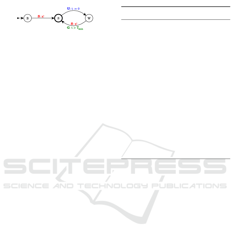
Figure 6: Non-deterministic input sequence automaton.

is ﬁred over channel y and the automaton moves to lo-

cation P, representing a silent period. After that, the

automaton proceeds with the encoding of Φ

B.2 Non-deterministic Input Sequences

Non-deterministic input sequences are valid input se-

quences where the occurrence times of spikes is ran-

dom but the minimum inter-spike quiescence duration

is T

min

. Such sequences can be generated by an au-

tomaton deﬁned as follows:

Deﬁnition 5 (Non-deterministic input generator).

A non-deterministic input generator I

is a tuple

(L,B,X , Σ,Arcs,Inv), with:

• L = {B, S, W}, with S urgent,

• X = {t}

• Σ = x

• Arcs = {(B,t = D,x!,

0,S), (S,true, ε,{t :=

0},W), (W,t > T

min

,x!,

0,S)}

• Inv(B) = (t ≤ D)

where D is the initial delay.

The behavior of such a generator depends on clock

t and broadcast channel x, and can be summarized as

follows: it waits in location B an arbitrary amount of

time before moving to location S, ﬁring its ﬁrst spike

over channel x. Since location S is urgent, the au-

tomaton instantaneously moves to location W, reset-

ting clock t. Finally, from location W, after an arbi-

trary amount of time t, it moves to location S, ﬁring

a spike. Notice that an initial delay D may be intro-

duced by adding the invariant t ≤ D to the location B

and the guard t = D on the edge (B → S).

C Additional Material for the

Advice Back-Propagation

Algorithm

Here we provide more details on the ABP algorithm:

the pseudo-code handling the update of the synaptic

weights and the propagation of advices is given in Al-

gorithms 1 and 2. In both algorithms, ∆ is a constant

factor used to manage increments and decrements.

Algorithm 2: Abstract ABP: Should Not Have Fired ad-

vice pseudo-code.

1: procedure SHOULD-NOT-HAVE-

FIRED(neuron)

2: if IS-VISITED(neuron) then

3: return

4: SET-VISITED(neuron, True)

5: for i ← 1 ... COUNT-

PREDECESSORS(neuron) do

6: weight

← GET-WEIGHT(neuron, i)

7: f ired

← FIRED-RECENTLY(neuron, i)

8: neuron

← GET-PREDECESSOR(neuron,

9: DECREASE-WEIGHT(neuron, i, ∆)

10: if weight

≥ 0 then

11: if f ired

then

12: SHOULD-NOT-HAVE-

FIRED(neuron

)

13: else

14: if ¬ f ired

then

15: SHOULD-HAVE-FIRED(neuron

)

 Advice propagation

BIOINFORMATICS 2018 - 9th International Conference on Bioinformatics Models, Methods and Algorithms