
Semi-supervised Distributed Clustering for Bioinformatics - Comparison
Study
Huayiing Li and Aleksandar Jeremic
Dept. of Electrical and Computer Engineering, McMaster University, Hamilton, Canada
Keywords:
Information Fusion, Bioinformatics, Distributed Clustering.
Abstract:
Clustering analysis is a widely used technique in bioinformatics and biochemistry for variety of applications
such as detection of new cell types, evaluation of drug response, etc. Since different applications and cells
may require different clustering algorithms combining multiple clustering results into a consensus clustering
using distributed clustering is a popular and efficient method to improve the quality of clustering analysis.
Currently existing solutions are commonly based on supervised techniques which do not require any a priori
knowledge. However in certain cases, a priori information on particular labelings may be available a priori. In
these cases it is expected that performance improvement can be achieved by utilizing this prior information.
To this purpose in this paper, we propose two semi-supervised distributed clustering algorithms and evaluate
their performance for different base clusterings.
1 INTRODUCTION
Mutation is an accidental change in genomic se-
quence of DNA (Pickett, 2006) and has been often
used in biochemistry in order to produce to improve
features of different objects such as plants, drugs, etc.
These changes are usually observed (monitored) us-
ing fluorescence microscopy, an important tool for vi-
sualizing biochemical activity within individual cells.
Automated analysis of these imagestypically involves
acquiring high resolution images and translating them
into a multi-dimensional feature space, which spans
hundreds of features per fluorescence channel and
will be further processed to provide relevant output
(Shariff et al., 2010) which is commonly done us-
ing clustering algorithms. Although there are many
clustering algorithms exist in the literature, no single
algorithm can correctly identify underlying structure
of all data sets in practice (Xu and Wunsch, 2008).
Combing multiple clusterings into a consensus label-
ing is a hard problem because of two reasons: (1)
number of clusters could be different and (2) label
correspondence problem. In (Vega-Pons and Ruiz-
Shulcloper, 2011), the authors provide a detailed re-
view of many existing algorithms: some algorithms
are based on relabeling and voting; some are based
on co-association matrix. All of these algorithms are
unsupervised learning because input data set is un-
labeled and clusters are not pre-defined. Also, most
of cluster ensemble algorithms consists of two ma-
jor steps: cluster ensemble generation and consensus
fusion. Different from the distributed detection prob-
lem, information fusion for cluster analysis is more
difficult because of at least the following two rea-
sons: (1) the number of clusters in each clustering
could be different and the desired number of clus-
ters is usually unknownand (2) the cluster labels from
different clusterings are symbolic and the same sym-
bolic label from different clusterings sometimes cor-
responds to different clusters. Therefore, a correspon-
dence problem is always accompanied with cluster-
ing ensemble problem (Strehl and Ghosh, 2003). The
common way to aviod the correspondence problem
(Dudoit and Fridlyand, 2003; Fred and Jain, 2005)
is to construct a pairwise similarity matrix between
data points. In (Strehl and Ghosh, 2003), the authors
proposed three algorithms based on hypergraph rep-
resentation of clusterings to solve the ensemble prob-
lem. In the meta-clustering algorithm (MCLA), the
clusters of a local clustering are represented by hyper-
edges. Many other approaches to combine the base
clustering have been proposed in the literature, such
as relabelling and voting based and mixture-densities
based approach.
In this paper we propose f two semi-supervise
clustering algorithms: soft and hard decision mak-
ing versions and compare their performances. For
the soft semi-supervised clustering ensemble algo-
rithm (SSEA), the average association vector is com-
Li H. and Jeremic A.
Semi-supervised Distributed Clustering for Bioinformatics - Comparison Study.
DOI: 10.5220/0006253502590264
In Proceedings of the 10th International Joint Conference on Biomedical Engineering Systems and Technologies (BIOSTEC 2017), pages 259-264
ISBN: 978-989-758-212-7
Copyright
c
2017 by SCITEPRESS – Science and Technology Publications, Lda. All rights reserved
259

puted for each data points and all the average associ-
ation vectors are normalized to derive the soft con-
sensus label matrix for the given data set. For the
hard semi-supervised clustering ensemble algorithm
(HSEA), the hard consensus clustering is generated
from two approaches. One approach is to assign each
data point its most associated cluster id based on its
average association vector. This version is named as
soft to hard semi-supervised clustering ensemble al-
gorithms (SHSEA). The other approach is to relabel
the set of base clusterings by assigning each data point
its most associated cluster id according to each base
clustering and to derive the hard consensus clustering
by majority voting. This is considered as hard to hard
semi-supervised clustering ensemble algorithm (HH-
SEA).
2 DISTRIBUTED CLUSTERING
In the literature, many clustering ensemble algo-
rithms have been proposed and can be broadly di-
vided into different categories, such as relabelling
and voting based, co-association based, hypergraph
based and mixture-densities based clustering ensem-
ble algorithms (Ghaemi et al., 2009), (Vega-Pons
and Ruiz-Shulcloper, 2011), (Aggarwal and Reddy,
2013). Clustering ensemble methods usually consist
of two major steps: base clustering generation and
consensus fusion. The set of base clusterings can be
generated in different ways, which has been discussed
in the previous section. In this section, we provide a
brief review of several consensus fusion methods.
2.1 Semi-supervised Clustering
Ensemble
In this paper we propose the semi-supervised algo-
rithm that utilizes the side information (data obser-
vations with known labels). The algorithm calcu-
lates the association between each data point and the
training clusters (formed by the labelled data observa-
tions) and relabels the cluster labels in Φ
u
according
to the training clusters. In the context of this paper,
since the generation of base clusterings is based on
unsupervised clustering algorithms and the fusion of
base clusterings is guided by the side information, we
name the proposed algorithm as the semi-supervised
clustering ensemble algorithm (SEA). It consists of
two major steps: the base clusterings generation and
fusion. The base clustering generation step is com-
mon to the exisiting ensemble methods and summa-
rized in Table 1. For the base clustering fusion step,
we propose different version of the fusion function
to produce soft and hard consensus clustering respec-
tively.
2.2 Soft Semi-supervised Clustering
Ensemble Algorithm
Suppose the input data set X is the combination of
a training set X
r
and a testing set X
u
. The training
set X
r
contains data points {x
1
,...,x
N
r
}, for which
labels are provided in a label vector λ
r
. The testing
data set X
u
contains data points {x
N
r
+1
,...,x
N
}, the
labels of which are unknown. The consensus clus-
ter label vector (output of SEA) for the test set X
u
is
denoted by λ
u
. The size of training set X
r
is the mea-
sure of the number of data points in the training set
and is denoted by N
r
, i.e., |X
r
| = N
r
. Similarly, the
size of testing set X
u
is the measure of the number
of data points in the testing set and is denoted by N
u
,
i.e., |X
u
| = N
u
. According to the training and testing
sets, the label matrix Φ can be partitioned into two
block matrices Φ
r
and Φ
u
, which contain all the la-
bels corresponding to the data points in the training
set X
r
and testing set X
u
respectively. Suppose train-
ing data points belong to K
0
classes and all training
points from the k-th class form one cluster, denoted
by C
k
r
(k = 1,...,K
0
). Therefore, the training set X
r
consists of a set of K
0
clusters {C
1
r
,...,C
k
r
,...,C
K
0
r
}.
If the size of cluster C
k
r
is denoted by N
k
r
, the total
number of training points N
r
is equal to
∑
K
0
k=1
N
k
r
. We
rearrange label matrix Φ
r
to form K
0
block matrices:
Φ
1
r
,...,Φ
k
r
,...,Φ
K
0
r
. Each block matrix Φ
k
r
contains
the base cluster labels of data points in the k-th train-
ing cluster C
k
r
where k = 1,...,K
0
.
For a given set of base clusterings, the soft version
of the semi-supervised clustering algorithm (SSEA)
has the ability to provide a soft consensus cluster label
matrix. The fusion idea is stated as follow: (1) for a
particular data point count the number of agreements
between its label and the labels of training points in
each training cluster, according to an individual base
clustering (2) calculate the association vector between
this data point and the corresponding base clustering,
(3) compute the average association vector by averag-
ing the association vectors between this data point and
all base clusterings and (4) repeat for all data points
and derive the soft consensus clustering for the testing
set. The summary of SSEA is provided in Table 2.
According to the j-th clustering λ
( j)
, we compute
the association vector a
( j)
i
for the i-th unlabelled data
point x
i
, where i = 1,...,N
u
and j = 1,...,D. Since
there are K
0
training clusters, the association vector
a
( j)
i
has K
0
entries. Each entry describes the asso-
ciation between data point x
i
and the corresponding
BIOSIGNALS 2017 - 10th International Conference on Bio-inspired Systems and Signal Processing
260

Table 1: Base clusterings generation.
* Input: Data set X
* Output: Base clusterings Φ
(a) Select clustering algorithm and determine its initialization and param-
eter settings to build clusterer φ
( j)
(b) Apply clusterer φ
( j)
to data set X and obtain individual clustering λ
( j)
(c) Repeat (a) and (b) for j = 1,...,D to form a set of base clusterings Φ
Table 2: Soft semi-supervised clustering ensemble algorithm (SSEA).
* Input: Base clusterings Φ
* Output: Soft clustering Λ
u
(a) According to label vector λ
r
, rearrange base clusterings Φ into K
0
+ 1 sub-
matrices {Φ
1
r
,...,Φ
k
r
,...,Φ
K
0
r
,Φ
u
}
(b) For data point x
i
, calculate the k-th element of the association vector a
( j)
i
by
a
( j)
i
(k) =
occurrence ofΦ
u
(i, j) inΦ
k
r
(:, j)
N
k
r
and repeat for k = 1,...,K
0
to form the association vector a
( j)
i
(c) Compute the average association vector a
i
of data point x
i
by a
i
=
1
D
∑
D
j=1
a
( j)
i
.
(d) Compute the association level γ
i
of data point x
i
to all training clusters by
γ
i
=
∑
K
0
k=1
a
i
(k).
(e) Compute the membership information of data point x
i
to every cluster by
normalizing a
i
(f) Repeat step (b) to (d) to generate the association level vector γ
u
and repeat
step (b) to (e) to generate the soft clustering Λ
u
training cluster. The k-th entry of the association vec-
tor a
( j)
i
is calculated by the ratio of occurrence of
Φ
u
(i, j) in Φ
k
r
(:, j) to the number of data points in the
k-th training cluster (N
k
r
), i.e.,
a
( j)
i
(k) =
occurrence ofΦ
u
(i, j) inΦ
k
r
(:, j)
N
k
r
, (1)
where Φ
u
(i, j) is the cluster label of data point x
i
ac-
cording to the j-th base clustering and Φ
k
r
(:, j) rep-
resents the labels of all data points in the k-th train-
ing category generated by the j-th local clusterer. For
each data point x
i
, different association vectors a
( j)
i
(j = 1,...,D) are calculated since there are D local
clusterers in the system. In order to fuse the informa-
tion, the avearge association vector a
i
for data point
x
i
is computed by averaging all the association vec-
tors a
( j)
i
, i.e.,
a
i
=
1
D
D
∑
j=1
a
( j)
i
. (2)
Each entry of a
i
describes the consolidated associ-
ation between data point x
i
and one of the training
clusters. As a consequnce, the summation of all the
entries of a
i
could be used to describe the associa-
tion between data point x
i
and all the training clusters
quantitively. We define it as the association level of
data point x
i
to all the training clusters and denote it
as γ
i
, i.e.,
γ
i
=
K
0
∑
k=1
a
i
(k). (3)
By computing the association levels for all the data
observations, the association level vector γ
u
for the
Semi-supervised Distributed Clustering for Bioinformatics - Comparison Study
261

Table 3: Soft to hard semi-supervised clustering ensemble algorithm (SHSEA).
* Input: Soft clustering Λ
u
* Output: Hard clustering λ
u
(a) Based on the average association vector a
i
, assign data point x
i
its most
assoicated cluster id, which corresponds to the highest entry in the average
association vector
(b) Repeat (a) for all i = 1,...,N
u
Table 4: Hard to hard semi-supervised clustering ensemble algorithm (HHSEA).
* Input: Base clusterings Φ
* Output: Hard clustering λ
u
(a) According to label vector λ
r
, rearrange base clusterings Φ into K
0
+ 1 sub-
matrices {Φ
1
r
,...,Φ
k
r
,...,Φ
K
0
r
,Φ
u
}
(b) For data point x
i
, calculate the k-th element of the association vector a
( j)
i
by
a
( j)
i
(k) =
occurrence ofΦ
u
(i, j) inΦ
k
r
(:, j)
N
k
r
and repeat for k = 1,...,K
0
to form the association vector a
( j)
i
(c) Assign data point x
i
its most associated cluster ids, which corresponds to
the highest entry of association vector a
( j)
i
(d) According to the j-th clustering, repeat step (b) and (c) for all data points
(e) Repeat (b) - (d) for j = 1,...,D and relabel Φ
u
into Φ
′
u
(f) Apply majority voting on Φ
′
u
to derive hard consensus clustering λ
u
testing set X
u
is made up by stacking association level
γ
i
for all i = 1,...,N
u
, i.e., γ
u
= [γ
1
,γ
2
,...,γ
N
u
]
T
. Let
us denote the soft consensus clustering of test set X
u
by a label matrix λ
u
. The i-th row of λ
u
is computed
by normalizing the average association vector a
i
, i.e.,
λ
u
(i,:) = a
T
i
/γ
i
. (4)
2.3 Hard Semi-supervised Clustering
Ensemble Algorithm
In this section, we propose the hard version of the
semi-supervised clustering ensemble algorithm from
two approaches. The first approaches is based on
calculating the average association vector a
i
for data
point x
i
. The consensus cluster label assigned to each
data point is its most associated category labels in the
corresponding average association vector. Since the
hard labels are derived from the soft label matrix Λ
u
,
it is named as the soft-to-hard semi-supervised clus-
tering ensemble algorithm (SHSEA). The summary of
this algorithm is provided in Table 3.
We also propose to derive hard consensus cluster-
ing from another approach. It is called hard to hard
semi-supervised clustering ensemble algorithm (HH-
SEA). The fusion idea stated as follow: (1) for a par-
ticular data point count the number of agreements be-
tween its label and the labels of training points in each
training cluster, according to an individual base clus-
tering, (2) calculate the association vector between
this data point and the corresponding base clustering,
(3) assign this data point to its most associated cluster
label (4) repeat for all data points and all base cluster-
ings to relabel the labels in matrix Φ
u
and (5) apply
majority voting to derive hard consensus clustering.
The summary of this algorithm is provided in Table 4.
3 NUMERICAL EXAMPLES
In this section, we provide numerical examples
to show the performance of our proposed semi-
supervised clustering ensemble algorithms: SHSEA
BIOSIGNALS 2017 - 10th International Conference on Bio-inspired Systems and Signal Processing
262
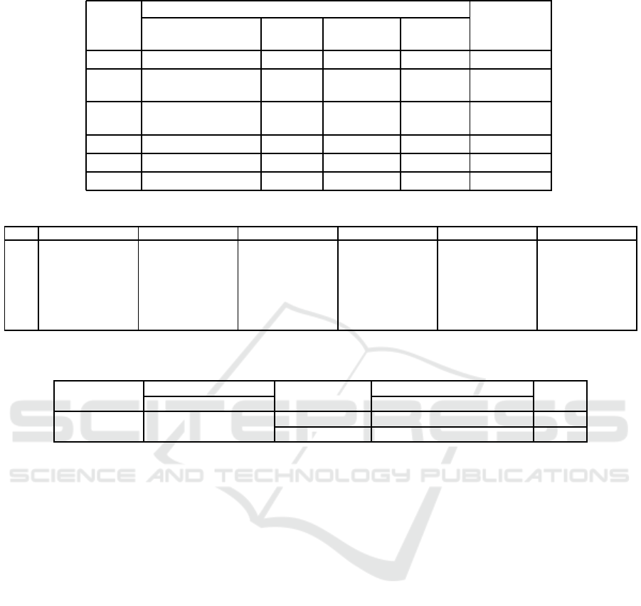
Table 5: Base Clusterings.
Individual base clustering No. of
Data
No. of Clustering No. of Base
features algorithms clusters Clusterings
Base 1 original F K-means k
( j)
> K
0
M
Base 2
Pre-processed
F
K-means/
k
( j)
> K
0
M
by PCA HAC/AP
Base 3
Pre-processed
F
pca
K-means
k
( j)
> K
0
M
by PCA
Base 4 original 1 K-means k
( j)
> K
0
F
Base 5 original 1 K-means k
( j)
= K
0
F
Base 6 original ⌈F/M⌉ K-means k
( j)
> K
0
M
Table 6: Average micro-precisions of SHSEA an HHSEA for different values of p using different sets of base clusterings.
p SHSEA HHSEA SHSEA HHSEA SHSEA HHSEA SHSEA HHSEA SHSEA HHSEA SHSEA HHSEA
3% 0.6351 0.4928 0.6282 0.4856 0.6363 0.4932 0.6374 0.3044 0.6150 0.3389 0.6282 0.4460
5% 0.6123 0.5170 0.6186 0.5150 0.6118 0.5162 0.6521 0.3838 0.6412 0.4570 0.6249 0.5139
10% 0.6530 0.5852 0.6551 0.5914 0.6558 0.5849 0.6645 0.5268 0.6521 0.5787 0.6702 0.6077
15% 0.6825 0.6269 0.6826 0.6324 0.6839 0.6277 0.7068 0.6072 0.7068 0.6974 0.6962 0.6455
20% 0.6900 0.6443 0.6830 0.6352 0.6933 0.6473 0.7275 0.6664 0.7264 0.6720 0.6983 0.6635
25% 0.7032 0.6579 0.7126 0.6636 0.7029 0.6578 0.7050 0.6659 0.6905 0.5879 0.7113 0.6848
30% 0.6868 0.6554 0.6918 0.6663 0.6866 0.6580 0.7274 0.6934 0.7232 0.6089 0.6994 0.6811
Table 7: Cancer data set: average micro-precisions of clustering algorithms (K-means, HAC and AP) on the original data sets
and the data pre-processed by PCA.
Data Sets
No. of
Dimensionality
Clustering Algorithms
MCLA
Data points Classes Kmeans HAC AP
3ClassesTest1 542 3
Original 705 0.4469 0.4299 0.4871 0.4989
PCA 100 0.4421 0.4354 0.5277 0.4487
and HHSEA using a real data set of breast cancer cells
undergoing treatment of different drugs. Since the ex-
pected cluster labels for each data set are available in
the experiments, we use micro-precision as our met-
ric to measure the accuracy of a clustering result with
respect to the expected labelling. Suppose there are k
t
classes for a given data set X containing N data points
and N
k
is the number of data points in the k-th cluster
that are correctly assigned to the corresponding class.
Corresponding class here represents the true class that
has the largest overlap with the k-cluster. The micro-
precision is defined by mp =
∑
k
t
k=1
N
k
/N (Wang et al.,
2011). We arbitrarily construct test files using data
points from different classes by randomly choosing
training data points. According to the values of p,
we randomly select the required number of training
points from their corresponding classes to form the
training file. For each value of p, we create 10 ver-
sions of training file for each test file and repeat the
experiment 10 time using each version of the training
file. For each value of p, we generate six sets of base
clusterings for each test file (note that test files refers
to different classes provided: original breast cancer
cells, cancer cells 24 hours after the drug treatment,
and cancer cells 72 hours after the drug treatment).
Since the dimensionality of the original data set is
quite large (705 features commonly used in biochem-
istry software packages), we generate an additional
set of base clusterings using different combinations
of the features to generate base clusterings instead of
using a single feature each time. The detailed infor-
mation about how to generate these sets of base clus-
terings is provided in Table 5. Note that K
0
is the
number of classes from which training points are se-
lected, F is the dimensionality of the feature space,
and F
pca
is the number of principle componentswhich
can retain 95% of the total variation of the original
data and M = 21 is used in the experiments. ⌈·⌉ rep-
resents the ceiling function. The micro-precisions are
listed in Table 6 in which the columns correspond to
base clusterings listed in the table.
REFERENCES
Aggarwal, C. C. and Reddy, C. K. (2013). Data clustering:
algorithms and applications. CRC Press.
Basu, S., Banerjee, A., and Mooney, R. (2002). Semi-
supervised clustering by seeding. In In Proceedings
Semi-supervised Distributed Clustering for Bioinformatics - Comparison Study
263

of 19th International Conference on Machine Learn-
ing (ICML-2002. Citeseer.
Chapelle, O., Sch¨olkopf, B., Zien, A., et al. (2006). Semi-
supervised learning.
Dudoit, S. and Fridlyand, J. (2003). Bagging to improve the
accuracy of a clustering procedure. Bioinformatics,
19(9):1090–1099.
Fred, A. L. and Jain, A. K. (2005). Combining multiple
clusterings using evidence accumulation. IEEE trans-
actions on pattern analysis and machine intelligence,
27(6):835–850.
Ghaemi, R., Sulaiman, M. N., Ibrahim, H., and Mustapha,
N. (2009). A survey: clustering ensembles techniques.
World Academy of Science, Engineering and Technol-
ogy, 50:636–645.
Liu, Y., Jin, R., and Jain, A. K. (2007). Boostcluster: Boost-
ing clustering by pairwise constraints. In Proceedings
of the 13th ACM SIGKDD international conference
on Knowledge discovery and data mining, pages 450–
459. ACM.
Pickett, J. P. (2006). The American heritage dictionary of
the English language. Houghton Mifflin.
Shariff, A., Kangas, J., Coelho, L. P., Quinn, S., and Mur-
phy, R. F. (2010). Automated image analysis for high-
content screening and analysis. Journal of biomolec-
ular screening, 15(7):726–734.
Strehl, A. and Ghosh, J. (2003). Cluster ensembles—
a knowledge reuse framework for combining multi-
ple partitions. The Journal of Machine Learning Re-
search, 3:583–617.
Vega-Pons, S. and Ruiz-Shulcloper, J. (2011). A survey of
clustering ensemble algorithms. International Jour-
nal of Pattern Recognition and Artificial Intelligence,
25(03):337–372.
Wang, H., Shan, H., and Banerjee, A. (2011). Bayesian
cluster ensembles. Statistical Analysis and Data Min-
ing, 4(1):54–70.
Xu, R. and Wunsch, D. (2008). Clustering, volume 10. John
Wiley & Sons.
BIOSIGNALS 2017 - 10th International Conference on Bio-inspired Systems and Signal Processing
264
