
Using Individual Feature Evaluation to Start Feature Subset Selection
Methods for Classification
Antonio Arauzo-Azofra
1
, Jos
´
e Molina-Baena
1
, Alfonso Jim
´
enez-V
´
ılchez
1
and Maria Luque-Rodriguez
2
1
Area of Project Engineering, University of Cordoba, Cordoba, Spain
2
Dept. of Computer Science and Numerical Analysis, University of Cordoba, Cordoba, Spain
Keywords:
Feature Selection, Attribute Selection, Attribute Reduction, Data Reduction, Search, Classification.
Abstract:
Using a mechanism that can select the best features in a specific data set improves precision, efficiency and the
adaptation capacity in a learning process and thus the resulting model as well. Normally, data sets contain more
information than what is needed to generate a certain model. Due to this, many feature selection methods have
been developed. Different evaluation functions and measures are applied and a selection of the best features is
generated. This contribution proposes the use of individual feature evaluation methods as starting method for
search based feature subset selection methods. An in-depth empirical study is carried out comparing traditional
feature selection methods with the new started feature selection methods. The results show that the proposal
is interesting as time gets reduced and classification accuracy gets improved.
1 INTRODUCTION
Inside the field of Pattern Recognition, the task of a
classifier is to use a feature vector to assign an object
to a category (Duda et al., 2000). A supervised classi-
fication learning algorithm generates classifiers from
a table of training vectors whose category is known.
However, sometimes these vectors have more features
than those really needed. Feature selection is a tech-
nique used in Machine Learning to choose a subset of
the available features that allows us to obtain accept-
able results, sometimes even better. This speeds up
the learning process by using less features.
The process of feature selection in any classifi-
cation problem is crucial since it allows us to elimi-
nate those features that may mislead us (the so-called
noise features), those features that do not provide
much information (irrelevant features) or those that
include repeated information (redundant characteris-
tics). Theoretically, if we knew the complete statisti-
cal distribution, the more features used the better re-
sults would be obtained. However, in practical learn-
ing scenarios, it might be better to use a feature set
(Kohavi and John, 1997).
Sometimes, if we have a large number of initial
features to analyze, the algorithms that are to carry out
this process may have memory or time consumption
problems or can even be turned inapplicable. The use
of feature selection functions may improve intelligi-
bility, the data acquisition costs and the manipulation
of data. Due to all these advantages, feature selection
has become a widely used technique in Data Mining.
As a result of this, several methods have been devel-
oped (Liu and Yu, 2005); (Thangavel and Pethalak-
shmi, 2009); (Tang et al., 2014). There are various ap-
plications of these methods, including, the prediction
of electricity prices (Amjady and Daraeepour, 2009),
classification of medical data (Polat and G
¨
unes, 2009)
or detection of intrusive systems.
We can distinguish the different parts of feature
selection using the modularization (Arauzo-Azofra
et al., 2011) shown in figure 1 (Arauzo-Azofra et al.,
2008). Almost every feature selection method can be
characterized through the evaluation method and the
search strategy employed.
There are two main types of feature selection al-
gorithms. One type is formed by those methods that
are based on a search strategy in the search space of
all possible feature sets together with a feature set
evaluation measure, which are commonly named fea-
ture subset selection methods (to emphasize that they
are working with sets). The other type is formed
by the methods that evaluate all features individu-
ally and then apply some cutting criteria to decide
which features are selected and which are not. On
one hand, feature subset selection methods are supe-
Arauzo-Azofra A., Molina-Baena J., JimÃl’nez-VÃ lchez A. and Luque-Rodriguez M.
Using Individual Feature Evaluation to Start Feature Subset Selection Methods for Classification.
DOI: 10.5220/0006204406070614
In Proceedings of the 9th International Conference on Agents and Artificial Intelligence (ICAART 2017), pages 607-614
ISBN: 978-989-758-220-2
Copyright
c
2017 by SCITEPRESS – Science and Technology Publications, Lda. All rights reserved
607
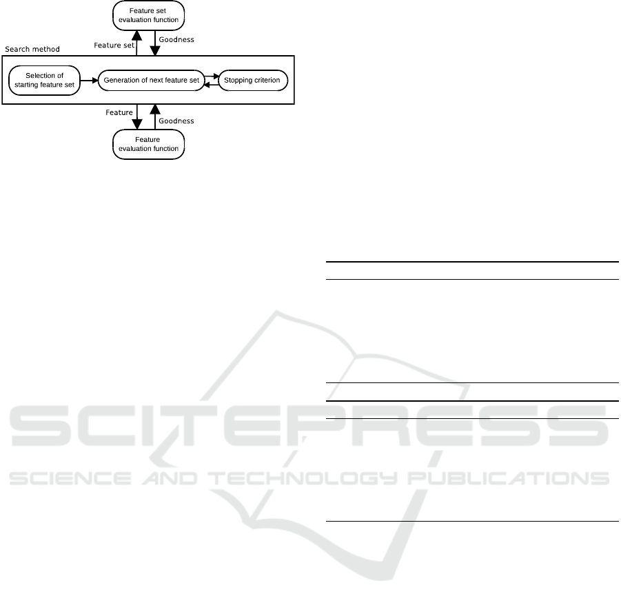
Figure 1: Feature selection modularized.
rior to those based on individual evaluation because,
as they can consider inter-dependencies among fea-
tures, they achieve better results. On the other hand,
individual feature selection methods are much faster
and easier to configure (Schiffner et al., 2016). These
are probably the reasons why they are so widely used.
Feature subset selection methods are slower be-
cause the search space is large (2
n
, being n the number
of features). For this reason, any improvement on the
search can be profitable. Focusing on the selection of
starting feature set module, the idea explored in this
paper is the hybridization of both types of feature se-
lection methods by using individual feature selection
methods as a starting method for the search strategy of
feature subset selection methods. With the hypothesis
that these combined methods can perform faster —as
they may avoid exploring some parts of the space—
and provide better features —by being focused on a
more concrete area of the space—, we compare tradi-
tional methods and the ones implementing the start-
ing strategy. This study help us to obtain conclusions
about how suitable individual evaluation methods are
to start feature subset selection methods.
This paper is organized as follows. In section 2,
feature selection methods are described. Section 3 de-
scribes in detail the proposed selection of starting fea-
ture sets . Section 4 describes the empirical method-
ology proposed to compare feature selection methods.
Finally, Sections 5 and 6 describe, respectively, the
results and the conclusions obtained.
2 FEATURE SELECTION
METHODS
The problem of feature selection may be seen as a
searching problem in the potential set of available fea-
tures set (Blum and Langley, 1997)(Kohavi, 1994).
The aim is to find a feature subset that allows us to
improve a learning process in any way.
2.1 Feature Subset Selection Methods
2.1.1 Search Methods
The search strategy for feature sets can be carried out
in different ways. In this contribution, several search
strategies are selected to have a great variety.
For the sequential search, the method Sequential
Forward Selection (SFS) and Sequential Backward
Selection (SBS) methods (Kohavi and John, 1997) are
selected. The former starts from an empty set of fea-
tures and it adds the feature that improve the selec-
tion the most, advancing towards the greatest valua-
tion near in the search space. The later is the reverse
because it conducts the search in the opposite direc-
tion.
Algorithm 1: SFS.
1: s
0
= {∅} Start with the empty set
2: loop:
3: x
+
= argmax[Score(s
k
+ x)];x /∈ s
k
Select the
best new feature
4: s
k+1
= s
k
+ x
+
;k = k + 1 Update
5: goto loop.
Algorithm 2: SBS.
1: s
0
= f eatures Start with the full set of features
2: loop:
3: x
−
= argmin[Score(s
k
−x)];x ∈Y
k
Select the
worse selected feature
4: s
k+1
= s
k
−x
−
;k = k + 1 Update
5: goto loop.
In probabilistic search, we can see algorithms that
follow some type of criterion that depends on some
random component. For this study, we have cho-
sen the search methods Las Vegas Filter (Liu and Yu,
2005) which is a filter probabilistic feature selection
algorithm designed for monotonic evaluation mea-
sures. This method involves random scan sets with
equal or lower number of features than the best one
found so far. Las Vegas Wrapper (Liu and Yu, 2005)
is similar but useful with non-monotonic measures as
in the wrapper approach.
As a representation of the meta-heuristic algo-
rithms, Simulated Annealing is used.
2.1.2 Measures of Feature Set Utility
Feature set measures are functions that, given a train-
ing data set (T ∈ >, every possible training sets are
called >) and a feature subset S ⊂ P(F) (P(F) de-
notes the powerset of F), return a valuation of the rel-
evance of those features.
ICAART 2017 - 9th International Conference on Agents and Artificial Intelligence
608

Algorithm 3: Las Vegas Filter.
1: Let s = features
2: for i = 0 to maxIterations do
3: s
new
= randomSubset(features, length(s))
4: if Score(s
new
) > Score(s) OR ( Score(s
new
) >
scoreThreshold AND length(s
new
) < length(s))
then
5: s ← s
new
6: i = i + 1
return s
Algorithm 4: Las Vegas Wrapper.
1: Let s = randomSubset(features)
2: for i = 0 to maxIterations do
3: s
new
= randomSubset(features)
4: if Score(s
new
) > Score(s) OR ( Score(s
new
) >
scoreThreshold AND length(s
new
) < length(s))
then
5: s ← s
new
6: i = i + 1
return s
Algorithm 5: Simulated Annealing.
1: Let s = s
0
2: for k = 0 to k
max
do
3: T ← temperature(k/k
max
)
4: s
new
← randomNeighbour(s)
5: if Prob(E(s),E(s
new
),T ) 6 random(0,1)
then
6: s ← s
new
7: k = k + 1
return s
Evaluation function : P(F) ×>→ R (1)
In our case, we have used three feature set mea-
sures which are described as follows:
• Inconsistent examples.
This measure uses an inconsistency rate that is
computed by grouping all examples (patterns)
with the same values in all of the selected features.
For each group, assuming that the class with the
largest number of examples is the correct class of
each group, the number of examples with a dif-
ferent class is counted (these are the inconsistent
examples) (Arauzo-Azofra et al., 2008). The rate
is computed dividing the sum of these counts by
the number of examples in the data set, as seen in
equation:
Inconsistency =
Number of inconsistent examples
Number of examples
(2)
In order to establish the relation between consis-
tency and inconsistency and since each one is de-
fined in the interval [0,1], we define the consis-
tency as:
Consistency = 1 −Inconsistency (3)
• Mutual information
This measure is based on the theory of informa-
tion by Shannon (Vergara and Est
´
evez, 2015). It
is defined as the difference between the class en-
tropy and the class entropy conditioned to know
the evaluated feature set. The aim of the learn-
ing algorithm is to reduce the uncertainty about
the value of the class. For this, the set of selected
features S provides the amount of the information
given by:
I(C,S) = H(C) −H(C|S) (4)
The ideal scenario would be to find the smallest
set of features that fully determine C, this means
I(C,S) = H(C), but it is not always possible.
• Wrapper approach measure
It uses the learning algorithm to evaluate whether
a data set is good. This measure uses a quality
measure obtained from the solutions of the learn-
ing algorithm. One of the advantages of this mea-
sure is that the feature selection algorithm per-
forms a feature evaluation in the real setting in
which it will be applied and thus it takes into ac-
count the possible bias of the learning algorithm
that is used.
2.2 Individual Feature Selection
Methods
2.2.1 Measures of Individual Feature Utility
The description of the five individual measures con-
sidered is as follows:
• Mutual Information (info) measures the quan-
tity of information that one feature gives about the
class (Vergara and Est
´
evez, 2015).
I(C,F) = H(C) −H(C|F) (5)
• Gain Ratio (gain) is defined as the ratio between
information gain and the entropy of the feature.
Gain ratio =
I(F,C)
H(F)
(6)
• Gini index (gini) can be seen as the probability of
two instances randomly chosen having a different
class. This measure is defined as follows:
Gini index =
∑
i, j∈C;i6= j
p(i|F)p( j|F) (7)
Using Individual Feature Evaluation to Start Feature Subset Selection Methods for Classification
609
• Relief-F (reli) is an extension of Relief
(Kononenko, 1994). It can handle discrete
and continuous attributes, as well as null values.
Despite evaluating individual features, Relief
takes into account relation among features. This
makes Relief-F to perform very well, becoming
well known and very commonly used in feature
selection.
• Relevance (rele) is a measure that discriminates
between attributes on the basis of their potential
value in the formation of decision rules (Dem
ˇ
sar
et al., 2013).
2.2.2 Cutting Criteria
In this study, we have used two cutting criteria. The
description of the two cutting methods chosen, fol-
lows.
• Fixed number (n) simply selects a given number
of a features. Obviously, the selected features will
be the ones with the greater evaluation.
• Fraction (p) selects a fraction, given as a percen-
tage, of the total number of available feature.
3 SELECTION OF STARTING
FEATURE SET
The proposal to test is the use of individual feature
selection methods embedded in search based feature
subset selection methods . These methods implement
an evaluation function that analyzes all the features
that represent the data set to be analyzed and after-
wards, a number of them are selected according to the
established criteria. These selected features will be
used as the feature set to start the search.
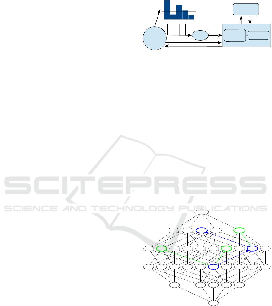
Figure 2, shows an schema of how starting method
works. As we can see, there are a set of initial features
{a, b, c, d, e} to which an evaluation function of indi-
vidual features is applied. Subsequently, the features
that have exceeded the cutting criteria of the individ-
ual measure are selected to form the starting method,
in our example the features would be {a, c, d}. With
these features initially selected, the search method ini-
tiates the search process to find the best possible set
of features.
Next, we will explain the process that each of the
search methods with starting set perform, for this we
will use a Hasse diagram where we represent the dif-
ferent movements performed by the algorithms in the
search space. The difference between the classical
and starting set methods is that the classical ones draw
from an empty initial starting set and the one with
a b c d e
a c d
Start set
Search method
Gen
erat
ion o
f
the n
ext
featu
re s
et
Stopping
criterion
Evaluation function
of feature sets
a b
c d
e
Cutting
Criterion
Figure 2: Starting method.
a starting set is no longer empty but starts with ini-
tial features that have been selected by the starting
method that we have implemented, as shown in fig-
ure 2.
In figure 3, we use blue to represent the sets that
are evaluated and selected as next; and we use green
to represent evaluated sets. In this example, SFS start
with a set of pre-selected features (the set containing
features b and d) and ends up selecting features a, b, d,
and e. Similarly, each of the search methods performs
different assessments of the following sets of features,
they choose one that meets the criteria established by
the algorithm. These iterations are performed until
the final set of features chosen by the algorithm are
reached.
Therefore, we can deduce that the new beginning
affects the reduction of time, as the number of assess-
ments are reduced in the selection of features, and so
the number of steps that the algorithm needs to get to
the final result.
a b c d e
a b c d a b c e a b d e a c d e b c d e
a b c a b d a c d b c da b e a c e b c ea d e b d e c d e
a b a c b ca d b da e b ec d c e d e
a b c d e
Figure 3: SFS with Start (Sequential Fordward Selection
with Start).
4 MATERIALS AND METHODS
In this section, we provide a detailed description of
the experimental methodology followed.
ICAART 2017 - 9th International Conference on Agents and Artificial Intelligence
610

4.1 Experimental Design
In the experiments performed in this study, the aim is
to compare each presented classic feature subset se-
lection method with its corresponding method started
using individual feature selection.
The dependent variables to evaluate the results of
feature selection are:
• The accuracy rate of classification (Acc).
• The number of selected features (Nof ).
• The time spent in feature selection (FSTime).
In order to get a reliable estimate of these vari-
ables, every experiment has been performed using 10-
fold cross-validation. For each experiment, we have
taken the mean and standard deviation of the ten folds.
In these experiments, there are several factors:
1. Starting method, with sub-factor:
• Cutting criterion
• Evaluation function of individual features
2. Feature subset selection method, with sub-factors:
• Search method
• Evaluation function of a set of features
3. Learning algorithm that generates the classifier.
4. Classification problem represented in a data set
(Data set).
The design of the global experiment is complete, in
order to subsequently be able to study the interactions
of all factors, alone or together. This means that all the
possible combinations among the factors are tested.
However, there are some exceptions with the Wrap-
per measure. It has not been tested with the larger data
sets (taking the size as the product of the number of
features by the number of examples): Adult, Anneal,
Audiology, Car, Ionosphere, led24, Mushrooms, Soy-
bean, Splice, Vehicle, Wdbc, Yeast, and Yeast-class-
RPR.
4.2 Data Sets
In order to include a wide range of classification
problems, the following publicly available reposito-
ries were explored seeking for representative prob-
lems with diverse properties (discrete and continu-
ous data, different number of classes, features, exam-
ples, and unknown values): UCI (Newman and Merz,
1998) and Orange (Dem
ˇ
sar et al., 2013). Finally, 36
data sets were chosen. They are listed along with their
main properties in Table 1:
• Data set column show the name by which data
sets are known.
• Ex. is the number of examples (tuples) in the data
set.
• Feat. is the number of features.
• Type of features: Discr. (all are discrete), Cont.
(all are continuous) or Mixed (both types).
• Cl. is the number of classes.
Table 1: Data sets used in experimentation.
Data set Ex. Feat. Type Cl.
Adult 32561 14 Mixed 2
Anneal 898 38 Mixed 5
Audiology 226 69 Discr. 24
Balance-Scale 625 4 Discr. 3
Breast-cancer 286 9 Mixed 2
Bupa (Liver Dis.) 345 6 Cont. 2
Car 1728 6 Discr. 4
Credit 690 15 Mixed 2
Echocardigram 131 10 Mixed 2
Horse-colic 368 26 Mixed 2
House-votes84 435 16 Discr. 2
Ionosphere 351 32 Cont. 2
Iris 150 4 Cont. 3
Labor-neg 57 16 Mixed 2
Led24-10000 10000 24 Discr. 10
Led24-1200 1200 24 Discr. 10
Lenses 24 4 Discr. 3
Lung-Cancer 32 56 Discr. 3
Lymphography 148 18 Discr. 4
M. B. Promoters 106 57 Discr. 2
Mushrooms (exp.) 8416 22 Discr. 2
Parity3+3 500 12 Discr. 2
Pima 768 8 Cont. 2
Post-operative 90 8 Mixed 3
Primary-tumor 339 17 Discr. 21
Saheart 462 9 Mixed 2
Shuttle-landing-c. 253 6 Discr. 2
Splice 3190 60 Discr. 3
Tic-tac-toe 958 9 Discr. 2
Vehicle 846 18 Cont. 4
Vowel 990 10 Cont. 11
Wdbc 569 20 Cont. 2
Wine 178 13 Cont. 3
Yeast 1484 8 Cont. 10
Yeast-class-RPR 186 79 Cont. 3
Zoo 101 16 Discr. 7
4.3 Classifiers
In order to estimate the quality of the feature selection
process executed by each method, the experiments are
performed in a full learning environment for classifi-
cation problems.
A set of well known methods have been consid-
ered. These methods have been chosen to cover each
category the most used methods belong to. They are:
Naive Bayes (NBayes), a simple probabilistic clas-
sifier; the K Nearest Neighbor (kNN), an algorithm
Using Individual Feature Evaluation to Start Feature Subset Selection Methods for Classification
611

based on the assumption that closer examples belong
to the same class; C4.5 (C45), a decision tree based
classification ; Multi-Layer Perceptron (ANN), an ar-
tificial neural network; and Support Vector Machine
(SVM), a set of supervised learning algorithms devel-
oped by Vladimir Vapnik.
4.4 Development and Running
Environment
The feature selection methods have been programmed
in Python. The software used for learning methods
has been Orange (Dem
ˇ
sar et al., 2013) component-
based data mining software, except for artificial neu-
ral networks, where SNNS (U. of Stuttgart,1995) was
used, integrated in Orange with OrangeSNNS pack-
age.
Experiments have run on a cluster of 8 nodes with
“Intel Xeon E5420 CPU 2.50GHz” processor and 2
nodes with ‘Intel Xeon E5630 CPU 2.53GHz”, under
Ubuntu 16.04 GNU/Linux operating system.
4.5 Parameters and Data
Transformations
All evaluation functions are parameter free except
Relief-F. For this measure, the number of neighbors
to search was set to 6, and the number of instances to
sample was set to 100.
Some of the learning algorithms require parameter
fitting. In the case of kNN, k was set to 15 after testing
that this value worked reasonably well on all data sets
used. The multi-layer perceptron used have one layer
trained during 250 cycles with a propagation value
of 0.1. For SVM we used Orange.SVMLearnerEasy
method to fit parameters to each case automatically.
Besides, consistency and information measures
require discrete valued features. For this reason, af-
ter some preliminary tests with equal frequency and
equal width discretization methods, we have chosen
the later with six intervals. This is only applied for
feature selection. Then learning algorithms get the
features with the original data.
5 EXPERIMENTAL RESULTS
This section presents the results according to the fol-
lowing scheme:
• Obtain the best individual measure and cutting
criterion to start each search method.
• The results comparing the classical methods and
the started methods.
5.1 Starting Method Set Up
The starting method have two parts:
• The initial evaluation function of individual fea-
tures.
• The cutting criterion. To carry out a selection of
the chosen parameters, we have taken into account
the best results obtained in (Arauzo-Azofra et al.,
2011). The parameters tested in each of the cut-
ting criteria are as follows:
– Fixed number (denoted as n-n) n ∈{9,13,17}
– Fraction (denoted as p-p) p ∈ 0.2, 0.5,0.8}
As we have five individual measures and six cut-
ting criterion possibilities, we have a total of thirty
options. Table 2 shows the best performing start-
ing method for each feature selection method —
according to its classification accuracy in the average
ranking among all data sets. As this has been done on
a varied set of data sets, we can recommend its use on
similar problems.
Table 2: Best parameter and individual measure for each
search method.
Search Parameters Individual measure
SFSwS n-17 gain
SBSwS n-17 info
LVFwS n-13 info
LVWwS n-17 gini
SAwS p-0.2 info
5.2 Comparisons Between Classical
Methods and Started Methods
Now, a series of comparisons between the classical
methods and the started ones will be conducted. We
draw from five classifiers (ANN, C4.5., KNN, N-
Bayes and SVM) and three set measures (Inconsistent
examples, Mutual Information and Wrapper). There-
fore, we will have a total of fifteen possible scenarios
to evaluate the success percentage, the number of fea-
tures and the feature selection time.
In the tables 3, 4, 5, 6 y 7, show the results
of Wilcoxon test confronting classic versus started
search methods applied with each combination of
the three measures and the five classifiers previously
shown. The tables indicate whether it is better the
classic method or the method with a starting set re-
flected in the Best column. On the other hand, they
indicate if the starting method significantly improves
the classical method, with a
√
(p-value < 0.10), or
if it does not improve significantly with – (p-value >
ICAART 2017 - 9th International Conference on Agents and Artificial Intelligence
612

Table 3: Wilcoxon test for methods SFS and SFS started.
Mea-Cla Best p-value Im.
IE-ANN started 0.011
√
IE-C4.5 started 0.003
√
IE-KNN started 0.459 –
IE-NBayes started 0.116 –
IE-SVM started 0.002
√
Inf-ANN started 0.144 –
Inf-C4.5 started 0.002
√
Inf-KNN started 0.020
√
Inf-NBayes started 0.132 –
Inf-SVM started 0.003
√
WRA-ANN started 0.875 –
WRA-C4.5 started 0.124 –
WRA-KNN started 0.469 –
WRA-NBayes classic 0.298 –
WRA-SVM started 0.755 –
Table 4: Wilcoxon test for methods SBS and SBS started.
Mea-Cla Best p-value Im.
IE-ANN started 0.068
√
IE-C4.5 started 0.256 –
IE-KNN started 0.370 –
IE-NBayes classic 0.835 –
IE-SVM started 0.042
√
Inf-ANN started 0.070
√
Inf-C4.5 started 0.218 –
Inf-KNN started 0.543 –
Inf-NBayes classic 0.438 –
Inf-SVM started 0.031
√
WRA-ANN started 0.233 –
WRA-C4.5 started 0.114 –
WRA-KNN started 0.347 –
WRA-NBayes classic 0.480 –
WRA-SVM started 0.041
√
Table 5: Wilcoxon test for methods LVF and LVF started.
Mea-Cla Best p-value Im.
IE-ANN started 0.830 –
IE-C4.5 classic 0.675 –
IE-KNN classic 0.909 –
IE-NBayes started 0.300 –
IE-SVM started 0.125 –
Inf-ANN started 0.088
√
Inf-C4.5 classic 0.241 –
Inf-KNN started 0.627 –
Inf-NBayes started 0.647 –
Inf-SVM started 0.014
√
0.10). In case the classical method improve its coun-
terpart with a starting set and this improvement is sig-
nificant it would have been indicated with X (p-value
Table 6: Wilcoxon test for methods LVW and LVW started.
Mea-Cla Best p-value Im.
WRA-ANN classic 0.722 –
WRA-C4.5 classic 0.285 –
WRA-KNN started 0.079
√
WRA-NBayes classic 0.4624 –
WRA-SVM started 0.979 –
Table 7: Wilcoxon test for methods SA and SA started.
Mea-Cla Best p-value Im.
IE-ANN started 0.149 –
IE-C4.5 started 0.005
√
IE-KNN started 0.014
√
IE-NBayes started 0.032
√
IE-SVM started 0.013
√
Inf-ANN started 0.330 –
Inf-C4.5 started 0.135 –
Inf-KNN started 0.313 –
Inf-NBayes started 0.110 –
Inf-SVM started 0.390 –
WRA-ANN started 0.110 –
WRA-C4.5 classic 0.499 –
WRA-KNN started 0.155 –
WRA-NBayes started 0.463 –
WRA-SVM classic 0.889 –
< 0.10). However this has not occurred in any case.
On every case in which classic perform better, the dif-
ference is not significant.
After analyzing the results, we can say that, gen-
erally, starting methods improve their counterparts in
the average ranking of both, the classification accu-
racy and the time spent in the feature selection. How-
ever, as an aside comment, we should say that this
does not happen with the number of the selected fea-
tures, where the starting methods do not always beat
their classical counterparts.
6 CONCLUSIONS
This contribution has structured and proposed the use
of individual feature selection methods as the starting
method for the search involved in feature subset selec-
tion methods. It has been systematically tested over
several well known feature selection methods on 36
classification problems and evaluated with five learn-
ing algorithms.
After the evaluation, we can conclude that the ac-
curacy achieved has improved or maintained in most
of the experiments carried out, while computing time
spent on feature selection reduces when using the
starting methods. In contrast, the results on the re-
Using Individual Feature Evaluation to Start Feature Subset Selection Methods for Classification
613

duction of the number of features selected are mixed,
when using Inconsistent Examples the number of fea-
tures seems to grow using started methods while when
using the Wrapper and Mutual Information measures,
the largest reduction of selected features is often car-
ried out by some started search methods.
As future work, we hope that this contribution will
open new opportunities for researching improvements
on many feature selection methods and that being on
a systematized way that may lead to many different
proposals but in a well organized development frame.
ACKNOWLEDGMENTS
This research is partially supported by projects:
TIN2013-47210-P of the Ministerio de Econom
´
ıa y
Competitividad (Spain), P12-TIC-2958 and TIC1582
of the Consejeria de Economia, Innovacion, Ciencia
y Empleo from Junta de Andalucia (Spain).
REFERENCES
Amjady, N. and Daraeepour, A. (2009). Mixed price and
load forecasting of electricity markets by a new iter-
ative prediction method. Electric power systems re-
search, 79(9):1329–1336.
Arauzo-Azofra, A., Aznarte, J. L., and Ben
´
ıtez, J. M.
(2011). Empirical study of feature selection meth-
ods based on individual feature evaluation for classi-
fication problems. Expert Systems with Applications,
38(7):8170 – 8177.
Arauzo-Azofra, A., Benitez, J. M., and Castro, J. L. (2008).
Consistency measures for feature selection. Journal
of Intelligent Information Systems, 30(3):273–292.
Blum, A. L. and Langley, P. (1997). Selection of relevant
features and examples in machine learning. Artificial
Intelligence, 97(1-2):245–271.
Dem
ˇ
sar, J., Curk, T., Erjavec, A.,
ˇ
Crt Gorup, Ho
ˇ
cevar, T.,
Milutinovi
ˇ
c, M., Mo
ˇ
zina, M., Polajnar, M., Toplak,
M., Stari
ˇ
c, A.,
ˇ
Stajdohar, M., Umek, L.,
ˇ
Zagar, L.,
ˇ
Zbontar, J.,
ˇ
Zitnik, M., and Zupan, B. (2013). Orange:
Data mining toolbox in python. Journal of Machine
Learning Research, 14:2349–2353.
Duda, R. O., Hart, P. E., and Stork, D. G. (2000). Pattern
Classification (2Nd Edition). Wiley-Interscience.
Kohavi, R. (1994). Feature Subset Selection as Search with
Probabilistic Estimates.
Kohavi, R. and John, G. H. (1997). Wrappers for feature
subset selection. Artificial Intelligence, 97:273–324.
Kononenko, I. (1994). Estimating attributes: Analysis and
extensions of relief. In Proceedings of the European
Conference on Machine Learning on Machine Learn-
ing, ECML-94, pages 171–182, Secaucus, NJ, USA.
Springer-Verlag New York, Inc.
Liu, H. and Yu, L. (2005). Toward integrating feature selec-
tion algorithms for classification and clustering. IEEE
Trans. on Knowl. and Data Eng., 17(4):491–502.
Newman, C. B. D. and Merz, C. (1998). UCI repository of
machine learning databases.
Polat, K. and G
¨
unes, S. (2009). A new feature selection
method on classification of medical datasets: Ker-
nel f-score feature selection. Expert Syst. Appl.,
36(7):10367–10373.
Schiffner, J., Bischl, B., Lang, M., Richter, J., Jones, Z. M.,
Probst, P., Pfisterer, F., Gallo, M., Kirchhoff, D.,
K
¨
uhn, T., Thomas, J., and Kotthoff, L. (2016). mlr
Tutorial. ArXiv e-prints.
Tang, J., Alelyani, S., and Liu, H. (2014). Feature Selec-
tion for Classification: A Review. In Data Classifica-
tion, Chapman & Hall/CRC Data Mining and Knowl-
edge Discovery Series, pages 37–64. Chapman and
Hall/CRC.
Thangavel, K. and Pethalakshmi, A. (2009). Dimension-
ality reduction based on rough set theory: A review.
Applied Soft Computing, 9(1):1 – 12.
Vergara, J. R. and Est
´
evez, P. A. (2015). A review of fea-
ture selection methods based on mutual information.
CoRR, abs/1509.07577.
ICAART 2017 - 9th International Conference on Agents and Artificial Intelligence
614
