
A Pipeline and Metric for Validation of Personalized Human Body
Models
Sukhraj Singh and Subodh Kumar
Computer Science Department, Indian Institute of Technology Delhi, New Delhi, India
Keywords:
Shape Descriptors, Human Body Models, Anatomy, Mesh Validation.
Abstract:
Advanced and personalized Human Body Models (HBM) are increasingly important in human centered indu-
stry design such as passive vehicular safety analysis, using finite element and other methods. Often accurate
HBMs are painstakingly constructed for median human dimensions, and then modified and re-sized using per-
sonalization algorithms for various applications. Personalization algorithms rely on various anthropometric
measurements, and sometimes manual intervention, to deform the median HBM. The quality of a personalized
model is often defined in terms of local properties such as aspect ratio of finite elements produced. In some
cases it is inferred by visual comparison with some ground truth model or by measuring the anthropometric
errors with respect to known values. We seek to define the quality of deformation in anatomically suitable
geometric terms, which can be automatically computed. To this end, we compare the deformed anatomical
surface meshes with that of the median mesh in a shape descriptor space. Shape comparison and matching is
a well studied area. The tools devised for the same are largely application dependent. We present pipeline and
a metric for validating anatomical surface meshes. It is a problem that has not been extensively studied, even
though general shape comparison and matching techniques abound. Our metric incorporates global and part
based shape signatures. The main contribution of our work is to explore techniques suitable for comparison of
anatomical meshes by non technical experts. We formulate a pipeline that needs minimal user intervention.
1 INTRODUCTION
With increasing use of Human Body Models (HBM)
in human centered industry design there is ongoing
effort to create more detailed advanced Finite Element
based Human Body Models (FE-HBM). FE-HBMs
are particularly important for injury prediction. In the
last decade there has been effort to create highly de-
tailed FE-HBMs for this purpose. Models like HU-
MOS (Robin, 2001), THUMS (Iwamoto et al., 2002)
and more recently GHBMC (Gayzik et al., 2011) are
some of the most popular HBMs in the domain of in-
jury biomechanics research.
Creation of a good quality FE-HBM from CT-scan
data is a tedious and time consuming task, which can
take many person-months. It usually requires manual
intervention and quality control can be challenging.
Due to these reasons FE-HBMs are generally avai-
lable in a standard occupant pose for a median di-
mension of a given population. However, it is really
important to predict the injury for subjects in non-
standard pose, and of non-median shape and size. To
solve this problem, deformation algorithms (Hwang
et al., 2016; Vezin and Verriest, 2005; CEESAR et al.,
2014) are used to automatically resize or personalize
a standard median template HBM within anatomical
constraints. Thus, these algorithms deform an HBM
known to be of a ‘good quality’ to a target HBM sa-
tisfying certain dimensional requirements. The tar-
get dimensions are in some cases derived from target
X-ray or CT-Scan images or from anthropometric in-
formation (Cheng et al., 1996) derived from statisti-
cal shape analysis of a population. Deformation can
be done on an individual anatomical volumetric mesh
of an organ or at the skin of FE-HBM, which con-
sequently deforms the internal anatomical meshes as
well. Again, it is critical that deformation leads to a
model of a ‘good quality’.
Our goal is to validate, or measure the quality of,
such a personalized FE-HBM. This could be done by
directly defining the notion of ‘good’ in mathemati-
cal terms. The general way of computing the quality
of a personalized FE-HBM in bio-mechanics com-
munity is by using distortion measures like scaled
Jacobian, skewness or aspect ratio of the finite ele-
ments and comparing these values with the baseline
160
Singh S. and Kumar S.
A Pipeline and Metric for Validation of Personalized Human Body Models.
DOI: 10.5220/0006176201600171
In Proceedings of the 12th International Joint Conference on Computer Vision, Imaging and Computer Graphics Theory and Applications (VISIGRAPP 2017), pages 160-171
ISBN: 978-989-758-224-0
Copyright
c
2017 by SCITEPRESS – Science and Technology Publications, Lda. All rights reserved

FE-HBM (Lalonde et al., 2013) and then manually
evaluating simulation results. It is also done by mea-
suring the errors in anthropometric measurements of
the personalized HBM or that of palpable landmarks
of internal organs with that of actual human (Poulard
et al., 2012) or by visual comparison with the baseline
HBM. An alternative or rather complementary way to
assess quality is by comparing the geometric proper-
ties of a surface mesh extracted from an anatomical
volumetric mesh with an accurate anatomically cor-
rect baseline surface mesh.
In computer graphics, 3D shapes are often repre-
sented as polygonal, or triangular, surface meshes.
Comparison and matching of two shapes is funda-
mental in shape analysis. With the advancement in
3D capture technologies there has been a continuous
expansion of shape databases. Consequently, signifi-
cant advances in shape analysis have been made in the
area of shape retrieval and shape matching. A large
number of global shape signatures have been introdu-
ced so as to have efficient and correct shape retrieval
(Iyer et al., 2005; Tangelder and Veltkamp, 2007).
The other important work in shape analysis is the
analysis of the property of a mesh after it has un-
dergone mesh processing algorithms like simplifica-
tion, smoothing, watermarking, compression or de-
formation. These processed meshes are often com-
pared with the original mesh using absolute measures
like dihedral angles or other distortion measures. Me-
trics like Minkowski distance or Hausdorff distance
are also used to find the difference between meshes
(Aspert et al., 2002; Cignoni et al., 1998). More re-
cently, metrics like MSDM2 by (Lavou, 2011) have
been introduced which are human perception oriented
distortion measures. However using such methods as-
sumes that the two meshes are in the same coordinate
space and fully aligned. There are other visualization
based comparison approaches where Gaussian curva-
ture or Mean curvature is used to color the mesh so as
to facilitate visual comparison of the mesh (Zhou and
Pang, 2001). This requires significant user interven-
tion due to the visual inspection involved.
Further, many shape analysis methods depend on
the kind of shape domains they are applied to, e.g.,
man-made shapes, natural shapes, CAD models, etc.
Human anatomy is one such domain where these
shape analysis methods have not been applied exten-
sively. Although there has been research focused in
the image domain for anatomical organs, 3D surface
mesh analysis of human anatomical organs is not well
explored.
In particular, in the anatomical context, some de-
formations are acceptable, even desirable, while ot-
hers are not. For example, lengthening or fattening
of a Femur bone is likely due to the target dimen-
sion. On the other hand, a bulging lesser trochanter
implies a poor deformation. Thus purely geometric
distance between a median mesh and a personalized
mesh would not suffice. Our research has lead us to
the set of local and global geometric features, each al-
ready found in the literature, which together provide
a usable metric to help guide the personalization al-
gorithm.
The main contribution of our work is a 3D anato-
mical surface mesh comparison pipeline and a quality
metric – two scalar values that provide a measure of
similarity between a template mesh and a deformed
candidate mesh. Again, the candidate mesh is not ex-
pected to ‘match’ the template mesh in the sense that
shape matching algorithms depend on. Rather, it is li-
kely to be non-linearly deformed. Our metric focuses
on the fact that ‘good’ meshes contain all anatomical
parts in the right configuration and of the right relative
dimensions. In order to compute such a metric, we
• Incorporate various geometric feature based sig-
natures for anatomical meshes validation.
• Implement a part-based mesh validation pipeline,
which considers the local part based features, and
relational features between adjacent parts.
• Model the mesh validation problem as a graph
matching problem.
• Coin a resultant validation metric, which consi-
ders the local, relational and global geometric fe-
atures.
• Test the devised pipeline and metric for 3D anato-
mical surface meshes.
The remainder of the paper is organized as fol-
lows: in Section 2 we present the various proces-
sing blocks of the pipeline, Section 3 provides details
about the segmentation algorithm used to find parts,
Section 4 provides detail about various shape signa-
tures used and also the formulation of graph. Further,
Section 5 provides details about the algorithm used
for finding correspondence with an optional segment
merge step detailed in Section 6 and Section 7 details
metric computation. Finally, in Section 8 we discuss
the results of the pipeline and Section 9 concludes
with limitations and future scope of work.
2 THE PIPELINE
In our work we have mainly used 3D surface mes-
hes of human skeletal system, primarily of the lower
limb region. On the basis of shape, anatomists bro-
adly classify the bones as a) Long bones b) Short bo-
nes c) Irregular bones and d) Flat bones (Gray, 2001).
A Pipeline and Metric for Validation of Personalized Human Body Models
161
A particular bone may further be classified into parts
based on its topography such as shaft, fovea, fossa,
neck, head, condyles, etc. These are essentially anato-
mical terms whose analogy would be parts like, cylin-
drical, depression, protruding, spherical, rough, etc.
However, a surface mesh, by construction, may not be
able to represent all such features of the bone, it de-
pends on the resolution of the mesh and the purpose
for which a mesh is constructed.
We envisage to incorporate geometric features that
cater to the above classification of bony anatomy. Fe-
atures based on Eigen values help us gain an insight
into the overall shape of a bone, the shape diame-
ter function (Gal et al., 2007) caters to variability in
shape, and shape index values based signature (Koen-
derink and van Doorn, 1992) considers detailed sur-
face characteristics of a bone. The work of (Lavou
et al., 2013) also tries to find an optimal metric by
linearly combining various metrics with weights pre-
dicted using machine learning techniques applied on
LIRIS Masking Database. They have used different
geometrical properties viz. dihedral angles, max and
min curvature. Also the database used for learning
did not have anatomical meshes and the resultant me-
tric is a global visual distortion metric. The details of
the signatures used in current research are explained
further in Section 4.
Further, the work of (Biederman, 1987) on recog-
nition by parts (RBC) suggests that humans tend to
recognize an object based on its parts, and this has
been exploited in various part based shape retrieval
algorithms (Theologou et al., 2014). The work by (Ji-
ang et al., 2013) also follows a part based matching
approach, using a signature based on eigenfunctions
of Leplace-Beltrami operator for CAD models. In
our present work, we also take this notion into con-
sideration and develop a metric that focuses on part
based signatures and relationships between parts as
well. The steps involved in metric computation are
explained next.
Let us consider two polygonal surface meshes P
A
and P
B
, where P
A
is the template mesh known to be
anatomically correct and P
B
is the candidate mesh to
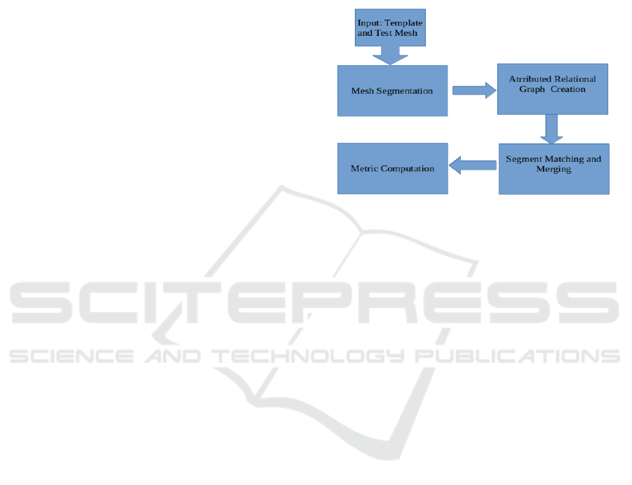
be validated. Figure 1 shows the main processing
blocks of pipeline and metric computation, the same
are described with some details as follows:
• Mesh Segmentation of the given two meshes,P
A
and P
B
.
• Attributed Relational Graph(ARG) creation from
the segmented meshes.
• Computation of cost matrix between the two
ARGs
• Computation of the segment to segment matching,
i.e., permutation matrix, using Hungarian node as-
signment algorithm.
• An Optional segment merging step, in case there
are unmatched segments.
• Finally, computation of global, part-based and re-
sultant mesh validation metric.
Figure 1: Pipeline Block Diagram.
The following sections provide the detail of the
above mentioned pipeline blocks.
3 MESH SEGMENTATION
In order to compute a part-based metric, the first step
is to compute these parts. We have chosen standard
segmentation to try to decompose a mesh into parts
as most anatomically salient parts indeed are geome-
trically also distinct from its neighbors. Although
segmentation is not our end goal and it is often suf-
ficient for the two meshes P
A
and P
B
to undergo si-
milar segmentation, we have found the Shape Dia-
meter Function (SDF) based segmentation algorithm
(Shapira et al., 2008) does well to align segments with
anatomical parts. The Princeton benchmark on 3D
mesh segmentation (Chen et al., 2009) ranks SDF ba-
sed segmentation algorithm as third in its evaluation
metric. Further, the SDF based segmentation takes
about 10x less time than the top two. The algorithm
is largely automatic: it does not need user intervention
to decide segment count. In fact, the default parame-
ters values mentioned by the authors generally work.
SDF is a volume based shape function and is in-
variant to rigid transformation and largely oblivious
to pose changes. It is defined as a scalar field on the
mesh surface and it gives a measure of the diameter
of the object’s volume in the neighborhood of each
point on the surface. It involves computation of a lo-
cal diameter at each vertex of a mesh. The histogram
GRAPP 2017 - International Conference on Computer Graphics Theory and Applications
162

of the SDF values is processed using Gaussian Mix-
ture Models and Expectation Maximization algorithm
to create consistent mesh partitions.
We use the implementation provided by the
CGAL library package (Yaz and Loriot, 2016) with
default values of 25 rays, cone angle of 120 degrees,
5 clusters and 0.26 as smoothing factor. We further
build upon the facet-id map provided as output of the
algorithm, to create separate polygon segment mes-
hes. These segment meshes are later used for creating
shape signatures in order to get the part-based compa-
rison metric.
We use the following notation. S
A
and S
B
are the
segmented polygonal meshes such that
S
A
=
n
[
i=1
S
ai
, S
ai
is the i
th
segment of mesh P
A
S
B
=
m
[
j=1
S
b j
, S
b j
is the j
th
segment of mesh P
B
Where, n and m are number of segments of P
A
and
P
B
, respectively.
4 ATTRIBUTED RELATIONAL
GRAPH CREATION
The segmented meshes S
A
and S
B
are used to cre-
ate two adjacency graphs. We create a node corre-
sponding to a segment and an edge for every pair of
adjacent segments of the segmented mesh. We as-
sociate properties a.k.a. attributes to the nodes and
the edges based on these segments, such a graph is
known as Attributed Relational Graph (ARG). The
Boost Graph Library (Siek et al., 2001) has been ex-
tensively used for the implementation of ARG. Let
G
A
= (V
a
, E
a
) be the ARG for the segmented mesh
S
A
and G
B
= (V
b
, E
b
) be the ARG for the segmented
mesh S
B
.
The node attributes are the signatures based on ge-
ometric shape descriptors of a mesh segment and the
edge attributes are the relational properties between
two adjacent mesh segments. The following subsecti-
ons provide details of the various geometric proper-
ties and thus signatures used to create these attributes.
We will use the terms node and segment interchange-
ably henceforth.
4.1 Node Attributes
Geometrical properties of segments that are assigned
to the nodes are termed as node attributes. The fol-
lowing subsection provide details of the various node
attributes used in our implementation.
4.1.1 SDF Signature
We create SDF signature of a segment, which is a log
normalized histogram of SDF values as described in
(Shapira et al., 2008).
nsd f =
log
sd f ( f )−min(sd f )
max(sd f )−min(sd f )
∗ η + 1
log(η + 1)
Where sd f : F → R is the SDF value for each facet
f and η is a normalizing parameter, which is set to 4.
The SDF signature is pose-oblivious and captures the
volumetric variation of a 3D shape. We use 64 bins to
create the histogram which is same as the original bin
count used by the authors in (Gal et al., 2007). Let us
denote, V
sd f
ai
and V
sd f
b j
, as the SDF signature for the
i
th
and the j
th
node of G
A
and G
B
, respectively.
4.1.2 Shape Index Signature
We create a Shape Index (SI) (Koenderink and van
Doorn, 1992) signature of a segment. which is a his-
togram of the SI values. If K
1
and K
2
are the principal
curvatures for a patch around a vertex of mesh, the SI
value for that patch is defined as:
si =
1
2
+
1
π
arctan
K
2
+ K
1
K
2
− K
1
, where K
1
6 K
2
The principal curvatures K
1
and K
2
are determi-
ned using the second order differential properties of
a local representation of the manifold fitted using a
jet, a truncated Taylor expansion (Cazals and Pouget,
2005). We use the CGAL library package by the same
authors (Pouget and Cazals, 2016) for estimating lo-
cal differential properties of a patch around a mesh
vertex via jet fitting.
The formula for determining SI values is changed
slightly from the original expression so that it is po-
sitive always. For all patches except the planar patch,
for which it is indeterminate, si ∈ [0, 1]. si is a scalar
that provides information about the shape of a patch,
e.g., whether it is a cup, cap, ridge, rut or saddle. Li-
kewise sdf signature, we use 64 bin histogram here as
well to create SI signature for a mesh segment. Let,
V
si
ai
and V
si
b j
, be the SI signature for the i
th
and the j
th
node of G
A
and G
B
, respectively.
4.1.3 Area Ratio
We compute the ratio of the area of a segment to the
area of the complete mesh. If Ar
S
is the surface area
of a mesh segment and Ar
P
the surface area of the
A Pipeline and Metric for Validation of Personalized Human Body Models
163

complete mesh, Area ratio accounts for the relative
size of each part.
α =
Ar
S
Ar
P
is defined as the area ratio of that segment. The same
is associated with the corresponding node of ARG.
Let, V
α
ai
and V
α
b j
, be the area ratio for the i
th
and the
j
th
node of G
A
and G
B
, respectively.
4.1.4 Eigen Value Based Shape Descriptor
If λ
1
, λ
2
and λ
3
are the three eigenvalues of a segment
s.t. λ
1
> λ
2
> λ
3
then the eigenvalues based shape
descriptor can be defined as in (Sidi et al., 2011):
e
1
=
λ
1
− λ
2
∑
3
i=1
λ
i
e
2
=
2(λ
2
− λ
3
)
∑
3
i=1
λ
i
e
3
=
3λ
3
∑
3
i=1
λ
i
We compute the eigenvalues based shape descrip-
tor as a vector having components e = < e
1
, e
2
, e
3
> of
each segment and assign it as an attribute to the cor-
responding node of the ARG. We use CGAL library
Principal Component Analysis package (Alliez et al.,
2016) to compute the eigenvalues of a mesh segment.
Let, V
e
ai
and V
e
b j
, be the shape descriptor for i
th
and j
th
node of G
A
and G
B
, respectively.
4.1.5 Node Degree
The node degree is the number of edges connected to
a node. Although this attribute is assigned to a node,
in strict sense it is a relational attribute. Let, V
deg
ai
and
V
deg
b j
be the node degree for the i
th
and the j
th
node of
G
A
and G
B
, respectively.
4.2 Edge Attribute
We compute a tuple that represents the angles bet-
ween the two largest eigenvectors (the ones with the
largest eigenvalues), respectively, of a segment with
its adjacent segment. If u
1s
is the largest and u
2s
the
next largest eigenvector of a segment S
A
and v
1s
and
v
2s
are similarly the two largest eigenvectors of an ad-
jacent segment S
B
, the tuple of eigenvector angles (in
radians) is defined as.
β
e
= [u
1s
− v
1s
, u
2s
− v
2s
]
This tuple is a relational feature that describes the
relative orientation of an adjacent segment to the gi-
ven segment. It is computed for all the edges incident
on an ARG node. Let, V
β
ai
and V
β
b j
, be the eigenvector
angle difference for the i
th
and the j
th
node of G
A
and
G
B
, respectively.
5 SEGMENT MATCHING
In this section we describe how to find for each seg-
ment of the candidate mesh, its corresponding seg-
ment in the template mesh. Finding corresponding
segments between segmented meshes S
A
and S
B
is a
two step process. First, a cost matrix C
nm
is compu-
ted, where n and m are the segment counts in S
A
and
S
B
, respectively. Each element of the cost matrix is
some form of distance between the two nodes in their
signature space. Second, this cost matrix is used to
obtain a node assignment using Harold Kuhn’s well-
known Hungarian Method for solving Optimal Assig-
nment Problems. The permutation matrix thus com-
puted is a boolean matrix with 1
0
s for the matched
nodes and 0
0
s for others. The following subsections
provide further details.
5.1 Cost Matrix Computation
Referring to the notations proposed in previous
section, the cost matrix for segmented mesh S
A
and
S
B
can be computed as follows:
loop: For all vertices a
i
of G
A
loop: For all vertices b
j
of G
B
c
sd f
i j
= EM D(V
sd f
ai
,V
sd f
b j
)
c
si
i j
= EM D(V
si
ai
,V
si
b j
)
c
α
i j
= L
1
(V
α
ai
,V
α
b j
)
c
e
i j
= L
2
(V
e
ai
,V
e
b j
)
c
deg
i j
= L
1
(V
deg
ai
,V
deg
b j
)
c
β
i j
= L
1
(V
β
ai
− V
β
b j
)
C
i j
= L
2
(c
sd f
i j
, c
si
i j
, c
e
i j
, c
α
i j
, c
deg
i j
, c
β
i j
)
endloop
endloop
Where, EMD is the earth movers distance (Rub-
ner et al., 1998). We use EMD to compute distance
between the signatures and absolute difference in case
of scalars. Each of the distances are normalized over
its range during the computation of the cost matrix
Table 1 gives the description of the notations used in
the pseudocode above.
5.2 Permutation Matrix Computation
We use libhungarian library (Gerkey, 2004) to solve
the node assignment problem. The cost matrix C
nm
described in section 5.1 is used for this computation.
We multiply Each element of the cost matrix with in-
teger 10, to just scale it, since the input to a libhun-
garian is supposed to be only integral values. The
Hungarian Algorithm produces a sparse permutation
GRAPP 2017 - International Conference on Computer Graphics Theory and Applications
164

Table 1: Notations used for the various cost/distance.
Notation
Description
c
sd f
i j
EMD between SDF
signatures
c
si
i j
EMD between SI signatures
c
α
i j
Absolute difference
between area ratio
c
e
i j
Euclidean distance between
shape descriptors
c
deg
i j
Absolute difference
between degrees
L
1
L1 norm
L
2
L2 norm
n × m sized matrix P
nm
, where P
i j
= 1 if i and j are
matching nodes.
6 SEGMENT MERGING
After completing the node assignment explained in
Section 5, some nodes of graph G
A
or G
B
may re-
main un-assigned. This happens when the number of
nodes in the two graphs are unequal. This could be
due to imperfect segmentation or some defect in the
candidate mesh. We consider the initial matching as
tentative in this case and iterate in an attempt to im-
prove the segmentation. In particular, we study the
impact on matching if we merge two adjacent seg-
ments. An improvement in matching is strongly sug-
gestive of imperfect segmentation and we finalize the
merger. The algorithm is listed in Algorithm 1. It may
happen that dist merge is greater than dist original in
all tentative merge cases, which results in ARGs ha-
ving unequal nodes even after the merge step. In that
case we use distance of the unmatched segment sig-
natures from zero valued signatures and consider that
as an added penalty in the metric computation.
G
M
is the resultant graph after the merge step.
We reapply the segment matching algorithm listed in
Section 5 between G
M
and the other graph. This again
results in a cost matrix and a permutation matrix. We
now use these two matrices to compute the part-based
metric as explained in following section.
7 METRIC COMPUTATION
The result of the segment matching step (see Sections
5 and 6) is the cost matrix C
nm
and the permutation
matrix P
nm
. The cost matrix C
nm
is a collation of the
distances of the segments in signature space. These
Algorithm 1: Segment Merging algorithm.
1: if num vertices(G
A
) > num vertices(G
B
) then
2: MERGESEGMENT(G
A
,G
B
);
3: else
4: MERGESEGMENT(G
B
,G
A
);
5: end if
6: function MERGESEGMENT ( G
X
,G
Y
)
7: for all Unmatched vertices V
u
in G
X
do
8: for all Neighbours V
nbr
of V
u
do
9: if V
nbr
is matched then
10: Merge V
nbr
and V
u
to get V
merge
11: Compute unary attributes of V
merge
12: Find distance dist merge between
V
merge
and corresponding vertex of V
nbr
in G
Y
13: if dist merge < dist original then
14: Keep the merge
15: else
16: Discard the merge
17: end if
18: end if
19: end for
20: end for
21: end function
Return the resultant graph after merging
return G
M
distances are EMD, Euclidean, Manhattan or Abso-
lute difference. An element C
i j
of matrix C
nm
is the
distance between segments i and j, respectively, of the
two meshes. As explained in Section 4, these node at-
tributes account for the segment shape and the edge
attributes account for the relation between segments.
The resultant metric is thus able to capture both the
part based shape and inter part relational aspect of the
meshes under comparison. Section 7.1 describes the
computation of complete part based metric. Section
7.2 describes the computation of the global metric.
7.1 Part-Based Metric
We use the computed cost matrix C
nm
(refer Section
5.1) and permutation matrix P
nm
(refer Section 5.2)
to compute the part based metric. We iterate through
P
nm
and check for matched nodes, and the correspon-
ding cost is picked from C
nm
. The L
2
norm of all these
costs is the computed part based metric. That is:
M
p
=
s
n
∑
i=1
m
∑
j=1
C
2
i j
P
i j
A Pipeline and Metric for Validation of Personalized Human Body Models
165

7.2 Global Metric
In order to compute the global metric, we first com-
pute the signature corresponding to the complete
mesh. We compute the SDF signature for the mes-
hes P
A
and P
B
and compute EMD between the two
signatures. If H
A
and H
B
are the histograms of SDF
values of the meshes P
A
and P
B
,
m
sd f
= EM D(H
A
, H
B
)
We also compute the eigenvalues based shape des-
criptor of the meshes as described in Section 4.1.4 for
mesh segments. If e
A
and e
B
are shape descriptors of
meshes P
A
and P
B
then,
m
e
=
q
e
2
A
− e
2
B
Lastly, we compute the SI values based global
shape signature of the meshes P
A
and P
B
(see Section
4.1.2). Thus if SI
A
and SI
B
are the histograms of SI
values of the meshes P
A
and P
B
,
m
si
= EM D(SI
A
, SI
B
)
We tested with both Euclidean distance and EMD
for histograms, and observed that EMD gives more re-
liable results in practice than does the Euclidean dis-
tance. This is due to the fact that EMD imparts a more
global sense to the distance between the two histo-
grams, whereas the Euclidean distance can be unduly
influenced by individual bins. For eigenvalues based
shape descriptor, which is not a histogram, we use the
Euclidean distance.
The resulting global metric is defined as the L
2
norm of m
sd f
, m
e
and m
si
:
M
g
=
q
m
sd f
2
+ m
e
2
+ m
si
2
7.3 Overall Metric
The final metric is reported as the pair of the part ba-
sed metric and the global metric, i.e.,
M
r
= (M
p
, M
g
)
Since both M
p
and M
g
are based on metrics like
EMD, Euclidean or Manhattan distances, the resul-
tant metric does follow non-negativity and symmetry
properties, but may not follow triangular inequality.
8 EXPERIMENTAL RESULTS
In section 8.1 we show an example validation for fe-
mur mesh having 16516 vertices and 33028 facets,
where the template femur mesh has been deformed
at the Lesser Trochanter region as shown in Figure
2. We shall discuss two examples: Example 1, where
the number of segments in the Template and the Test
meshes are the same, and Example 2, where the num-
ber of segments of the Template and Test meshes are
different. In the latter case, the mesh that has more
segments will undergo automatic merging based on
the algorithm as described in Section 6 The experi-
ment was carried out on a system having Processor:
Intel i7 CPU@2.40GHz and RAM: 8 GiB.
8.1 Example 1
Figure 5 shows the segmentation results of the tem-
plate mesh and the deformed test mesh at the Lesser
Trochanter region. It can be observed that for the gi-
ven parameters of the segmentation algorithm, it is
able to segment the femur into anatomically relevant
regions like a) Head b) Shaft c) Condylar region and
d) Greater trochanter. The results of the segmenta-
tion can change with the supplied parameters. In the
current example the test mesh has the same number
of segments as does the template mesh. The ARGs
are constructed from the segmented meshes, Figure 3
and Figure 4 show the obtained cost and permutation
matrices, respectively. Matching colors in Figure 5
represent the matched segments obtained in this step.
The cost and permutation matrices are used to
compute the part-based metric and the global metric.
The resultant metric is the pair of part-based and glo-
bal metric as explained in section 7.
M
p
= 13.5712 (1)
M
g
= 0.1307 (2)
M
r
= (13.5712, 0.1307) (3)
where, M
p
, M
g
and M
r
are the part-based, global
and resultant metrics, respectively. where, M
p
, M
g
and M
r
are the part-based, global and resultant me-
trics, respectively. The complete process took approx-
imately 43 seconds.
8.2 Example 2
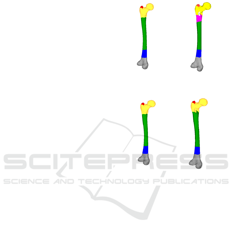
Figure 10 shows the segmentation results of the the
template mesh and test mesh deformed at the same
location, but by a larger amount, as that in the mesh
in Example 1. The segmentation algorithm, for the
same parameters produces seven segments in this
case. Thus the test mesh undergoes a merger step. Fi-
gure 6 and Figure 7 show the obtained cost matrix and
permutation matrix respectively. The matched seg-
ments in Figure 10 are shown in the same color. No-
tice that there are two unmatched segments, colored
GRAPP 2017 - International Conference on Computer Graphics Theory and Applications
166
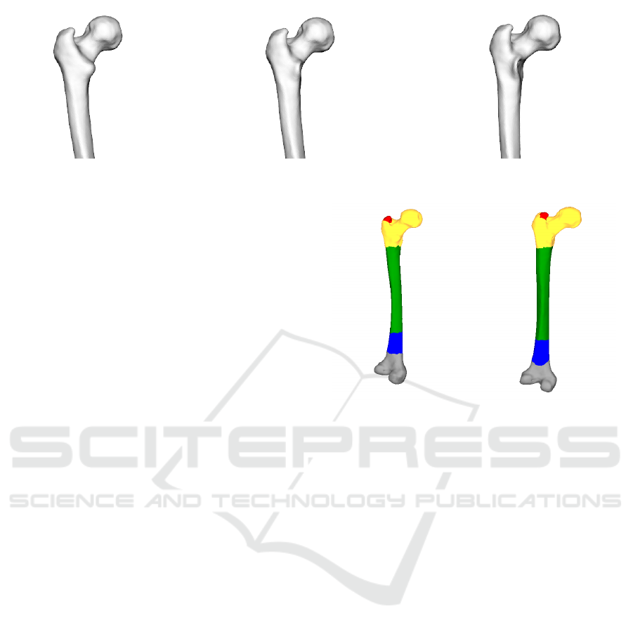
Figure 2: Femur Deformed at Lesser Trochanter: Template Mesh - Test Mesh 1 - Test Mesh 2.
10 39 23 25 41
40 2 29 27 25
25 32 6 20 34
33 29 18 1 26
44 26 27 22 5
Figure 3: 5 × 5 cost matrix femur example 1.
1 0 0 0 0
0 1 0 0 0
0 0 1 0 0
0 0 0 1 0
0 0 0 0 1
Figure 4: 5 × 5 permutation matrix computed femur exam-
ple 1.
pink and white. The complete process took approxi-
mately 42 seconds.
Figure 8 and Figure 9 show the obtained cost ma-
trix and permutation matrix after merging. Figure 11
shows the matched segments finally obtained in this
step. Notice that the two unmatched segments (from
Figure 10) are merged with their neighbouring seg-
ments in this step.
The cost and permutation matrices are used to
compute the part-based metric and the global metric.
These are then joined to produce the resultant metric
as explained in section 7.
M
p
= 19.2116 (4)
M
g
= 0.1347 (5)
M
r
= (19.2116, 0.1347) (6)
Clearly, in this case output global as well as part
based metric has greater value as compared to the ex-
ample 1 results, thus indicating a greater amount of
deformation. The merge step with computation of
metric took approximately 27 seconds.
Figure 5: Corresponding segments of Template and Test
Mesh 1.
24 7 39 31 21 29 33
33 33 5 34 29 23 21
24 21 30 27 7 22 23
29 24 24 33 19 5 17
37 36 21 32 32 19 12
0 0 0 0 0 0 0
0 0 0 0 0 0 0
Figure 6: 7 × 7 cost matrix Femur case 2.
8.3 Survey Results
We conducted a survey to check the efficacy of the
pipeline and the metric. The survey comprised ima-
ges of five different sets of meshes. Each set had
four meshes: one original template mesh and three
deformed versions of it. Side-on snapshots of each
mesh from four mutually perpendicular viewing an-
0 1 0 0 0 0 0
0 0 1 0 0 0 0
0 0 0 0 1 0 0
0 0 0 0 0 1 0
0 0 0 0 0 0 1
1 0 0 0 0 0 0
0 0 0 1 0 0 0
Figure 7: 7 × 7 permutation matrix Femur example 2.
A Pipeline and Metric for Validation of Personalized Human Body Models
167
7 45 20 27 36
37 11 31 24 20
24 40 8 21 27
28 32 20 5 21
40 28 32 20 8
Figure 8: 5 × 5 cost matrix femur example 2 after merge.
1 0 0 0 0
0 1 0 0 0
0 0 1 0 0
0 0 0 1 0
0 0 0 0 1
Figure 9: 5 × 5 permutation matrix femur example 2 after
merge.
gles were shown for evaluation. The three deformed
meshes in each set all had deformations at the same
location but with varying magnitudes. One of the sets
include deformed mesh output from a GEBOD based
(CEESAR et al., 2014; Cheng et al., 1996) FE-Mesh
personalization algorithm. A group of ten experts,
which comprised bio-mechanic researchers and medi-
cal practitioners, were asked to compare each defor-
med mesh (on the basis of the four snapshots) to the
template mesh and assign a rank from 1 to 3 indica-
ting the degree of deformation in their judgement. Fi-
gure 12 shows the results of the ranking marked by the
surveyors. There was significant agreement among
them.
We also computed the part-based and global me-
trics of the same set of deformed test meshes (with re-
spect to their respective templates). In Figure 13 and
Figure 14, we show the computed global and part-
based metrics, respectively.
We evaluate the metric against the survey. From
the survey, the modal rank of each deformed mesh
was taken as its anatomically standard rank. The ran-
kings from the metric were obtained directly: a hig-
her value of the metric implied a lower rank. Fi-
gure 15 shows the results of the comparison. Furt-
her, the surveyors were also asked to judge the ana-
tomical correctness of each test mesh by comparing
it to the corresponding template meshes. Specifi-
cally, the question was ”Are the two bones anatomi-
cally the same?”, to which they had to answer as a)
Strongly agree b) Agree c) Disagree or d) Strongly
disagree. We computed a cumulative-score for a par-
ticular answer as
∑
4
i=1
weight
i
∗ mode
i
, where weights
were assigned from 1 − 4 with 1 for ‘strongly agree’
and so on. It was observed that the correlation bet-
ween cumulative-score and part-based metric is signi-
ficant with correlation coefficient = 0.724. The corre-
lation coefficient between rankings and global-metric
is 0.900 and between rankings and part-based metric
Figure 10: Corresponding segments of Template and Test
Mesh 2 with two unmatched segments in color pink and
white.
Figure 11: Corresponding segments of Template and Test
Mesh 2 – Merged.
is 0.500.
Out of the five sets, the part-based metric dis-
agrees with the standard ranking of the first mesh and
the fifth mesh. For the first mesh, which is quite sym-
metric with similar shapes for opposite ends of mes-
hes under comparison, matching failed, in part due
to the segmentation. The sphere-like lateral condy-
lar region was segmented for the template mesh but it
matched the femoral head segment of the test mesh.
These had similar geometric and relational features,
and ended up in an inverse segment match. One way
to improve this is to use different parameters for the
segmentation algorithm and break symmetry. Since
we wanted the same parameter for all meshes, we did
not explore this further.
The fifth set had a torsion deformation at the fe-
mur condylar region. It was observed that the se-
cond mesh in this set had an equal number of seg-
ments to that of the template mesh. But the first mesh
had an unequal number of segments. Even though
the segment merging algorithm accounts for this dis-
crepancy, this case results in significant variations in
GRAPP 2017 - International Conference on Computer Graphics Theory and Applications
168
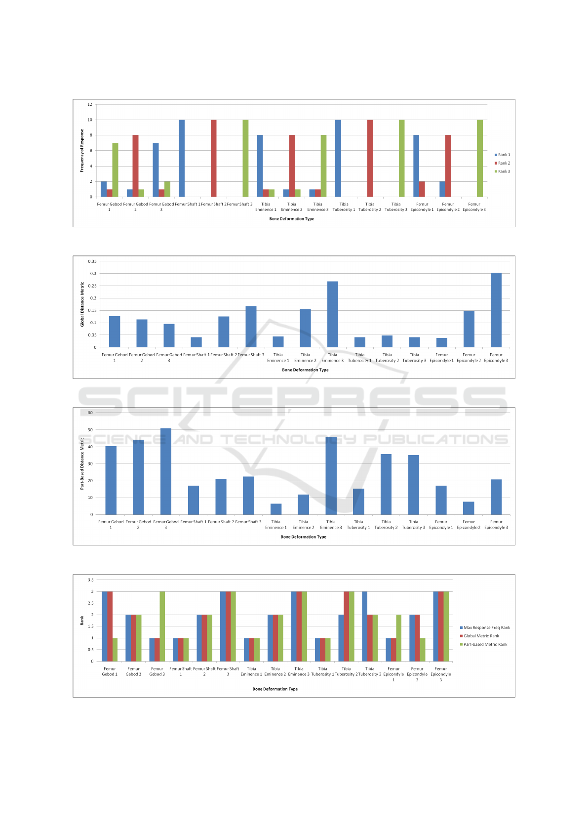
Figure 12: Ranking of Bone Deformation based on a Survey.
Figure 13: Deformed Mesh Global Metric.
Figure 14: Deformed Mesh Part-based Metric.
Figure 15: Comparison of Rankings based on a Survey, Global Metric and Part-Based Metric.
A Pipeline and Metric for Validation of Personalized Human Body Models
169

the segment boundaries, leading to deviations in the
computed metric. Overall, three cases out of five had
rankings identical to the survey’s for the part-based
metric and the other two cases had partly similar ran-
king, but in these case, the global metric had ranking
almost identical to the survey’s.
In particular, one might conclude that if both part-
based and global metrics indicate that a test-mesh has
a high rank, it is indeed of good anatomical quality.
9 CONCLUSION AND FUTURE
WORK
In this paper, we present a pipeline for the valida-
tion of personalized/deformed anatomical meshes by
comparing these with known correct meshes. The pi-
peline considers part-based, relational and global ge-
ometrical features and gives a resultant validation me-
tric. The complete pipeline requires little user inter-
vention and computes the validation metric in an au-
tomatic way. The efficacy of the validation metric
depends on three important factors, a) segmentation
algorithm b) the choice of geometric features or sig-
natures and c) the distance metric. We observed that
SDF based segmentation algorithm gives satisfactory
mesh partitions in case of anatomical organs. Howe-
ver, the segmentation output varies with the change in
parameters provided to the algorithm. Further inves-
tigation is needed to determine if a better segmenta-
tion into actual anatomical parts can improve the ma-
tch metric further. In further work, one may provide
some control to segment the template as a one time
effort. The candidate mesh can then be automatically
co-segmented with the template. In future, one can
test for additional signatures, anatomical meshes of
upper body region and improve on limitations of the
metric.
ACKNOWLEDGEMENTS
We thank our colleagues and institutions involved in
PIPER project (CEESAR et al., 2014) for providing
us access to the Anatomical Surface Mesh Data Set
and GHBMC model. Also, all the volunteers who
helped in filling the on-line survey for subjective tes-
ting. Further, the comments from anonymous revie-
wers have been very helpful.
REFERENCES
Alliez, P., Pion, S., and Gupta, A. (2016). Principal compo-
nent analysis. In CGAL User and Reference Manual.
CGAL Editorial Board, 4.9 edition.
Aspert, N., Santa-Cruz, D., and Ebrahimi, T. (2002). Mesh:
measuring errors between surfaces using the hausdorff
distance. In Multimedia and Expo, 2002. ICME ’02.
Proceedings. 2002 IEEE International Conference on,
volume 1, pages 705–708 vol.1.
Biederman, I. (1987). Recognition-by-components: A the-
ory of human image understanding. Psychological Re-
view, 94:115–147.
Cazals, F. and Pouget, M. (2005). Estimating differential
quantities using polynomial fitting of osculating jets.
Computer Aided Geometric Design, 22(2):121 – 146.
CEESAR, INRIA, U. et al. (2014). Position and Persona-
lize Advanced Human Body Models for Injury Pre-
diction. http://www.piper-project.eu/. [Online; acces-
sed 18-October-2016].
Chen, X., Golovinskiy, A., and Funkhouser, T. (2009). A
benchmark for 3d mesh segmentation. In ACM SIG-
GRAPH 2009 Papers, SIGGRAPH ’09, pages 73:1–
73:12, New York, NY, USA. ACM.
Cheng, H., Obergefell, L., and Rizer, A. (1996). The de-
velopment of the gebod program. In Biomedical En-
gineering Conference, 1996., Proceedings of the 1996
Fifteenth Southern, pages 251–254.
Cignoni, P., Rocchini, C., and Scopigno, R. (1998). Me-
tro: Measuring error on simplified surfaces. Computer
Graphics Forum, 17(2):167–174.
Gal, R., Shamir, A., and Cohen-Or, D. (2007). Pose-
oblivious shape signature. IEEE Transactions on Vi-
sualization and Computer Graphics, 13(2):261–271.
Gayzik, F. S., Moreno, D. P., Vavalle, N. A., Rhyne, A. C.,
and Stitzel, J. D. (2011). Development of the global
human body models consortium mid-sized male full
body model. Injury Biomechanics Research, pages
39–12.
Gerkey, B. P. (2004). C Implementation of the Hun-
garian Method. http://robotics.stanford.edu/ ger-
key/tools/hungarian.html. [Online; accessed 14-July-
2016].
Gray, H. (2001). Anatomy of the human body. Phi-
ladelphia: Lea & Febiger, 1918; Bartleby.com,
2000. http://www.bartleby.com/107/17.html. [Online;
accessed 18-October-2016].
Hwang, E., Hallman, J., Klein, K., Rupp, J., Reed, M., and
Hu, J. (2016). Rapid development of diverse human
body models for crash simulations through mesh mor-
phing. Technical report, SAE Technical Paper.
Iwamoto, M., Kisanuki, Y., Watanabe, I., Furusu, K., Miki,
K., and Hasegawa, J. (2002). Development of a fi-
nite element model of the total human model for sa-
fety (thums) and application to injury reconstruction.
In Proceedings of the International Research Council
on the Biomechanics of Injury conference, volume 30,
pages 12–p. International Research Council on Bio-
mechanics of Injury.
Iyer, N., Jayanti, S., Lou, K., Kalyanaraman, Y., and Ra-
mani, K. (2005). Three-dimensional shape searching:
GRAPP 2017 - International Conference on Computer Graphics Theory and Applications
170

state-of-the-art review and future trends. Computer-
Aided Design, 37(5):509 – 530. Geometric Modeling
and Processing 2004.
Jiang, L., Zhang, X., and Zhang, G. (2013). Partial
shape matching of 3d models based on the laplace-
beltrami operator eigenfunction. Journal of Multime-
dia, 8(6):655–661.
Koenderink, J. J. and van Doorn, A. J. (1992). Surface shape
and curvature scales. Image and Vision Computing,
10(8):557 – 564.
Lalonde, N. M., Petit, Y., Aubin, C.-E., Wagnac, E.,
and Arnoux, P.-J. (2013). Method to geometrically
personalize a detailed finite-element model of the
spine. IEEE Transactions on Biomedical Engineer-
ing, 60(7):2014–2021.
Lavou, G. (2011). A multiscale metric for 3d mesh vi-
sual quality assessment. Computer Graphics Forum,
30(5):1427–1437.
Lavou, G., Cheng, I., and Basu, A. (2013). Perceptual qua-
lity metrics for 3d meshes: Towards an optimal multi-
attribute computational model. In 2013 IEEE Interna-
tional Conference on Systems, Man, and Cybernetics,
pages 3271–3276.
Pouget, M. and Cazals, F. (2016). Estimation of local diffe-
rential properties of point-sampled surfaces. In CGAL
User and Reference Manual. CGAL Editorial Board,
4.9 edition.
Poulard, D., Bermond, F., Dumas, R., Bruyere, K., and
Compigne, S. (2012). Geometrical personalisation
of human fe model using palpable markers on volun-
teers. Computer methods in biomechanics and biome-
dical engineering, 15(sup1):298–300.
Robin, S. (2001). Humos: human model for safety–a joint
effort towards the development of refined human-like
car occupant models. In 17th international technical
conference on the enhanced safety vehicle, page 297.
Rubner, Y., Tomasi, C., and Guibas, L. J. (1998). A metric
for distributions with applications to image databases.
In Computer Vision, 1998. Sixth International Confe-
rence on, pages 59–66.
Shapira, L., Shamir, A., and Cohen-Or, D. (2008). Con-
sistent mesh partitioning and skeletonisation using
the shape diameter function. The Visual Computer,
24(4):249–259.
Sidi, O., van Kaick, O., Kleiman, Y., Zhang, H., and Cohen-
Or, D. (2011). Unsupervised co-segmentation of a
set of shapes via descriptor-space spectral clustering.
ACM Trans. on Graphics (Proc. SIGGRAPH Asia),
30(6):126:1–126:10.
Siek, J. G., Lee, L.-Q., and Lumsdaine, A. (2001). Boost
Graph Library: User Guide and Reference Manual,
The. Pearson Education.
Tangelder, J. W. H. and Veltkamp, R. C. (2007). A survey of
content based 3d shape retrieval methods. Multimedia
Tools and Applications, 39(3):441.
Theologou, P., Pratikakis, I., and Theoharis, T. (2014). A
review on 3d object retrieval methodologies using a
part-based representation. Computer-Aided Design
and Applications, 11(6):670–684.
Vezin, P. and Verriest, J. P. (2005). Development of a set of
numerical human models for safety. In 19th Internati-
onal Technical Conference on the Enhanced Safety of
Vehicles, Washington DC, pages 6–9.
Yaz, I. O. and Loriot, S. (2016). Triangulated surface mesh
segmentation. In CGAL User and Reference Manual.
CGAL Editorial Board, 4.9 edition.
Zhou, L. and Pang, A. (2001). Metrics and visualization
tools for surface mesh comparison. In Visual Data
Exploration and Analysis VIII, 99 (May 3, 2001), vo-
lume 4302, pages 99–110.
A Pipeline and Metric for Validation of Personalized Human Body Models
171
