
Joint Large Displacement Scene Flow and Occlusion Variational
Estimation
Roberto P. Palomares, Gloria Haro and Coloma Ballester
Universitat Pompeu Fabra, Barcelona, Spain
Keywords:
Scene Flow, Variational Methods, Coordinate Descent, Sparse Matches.
Abstract:
This paper presents a novel variational approach for the joint estimation of scene flow and occlusions. Our
method does not assume that a depth sensor is available. Instead, we use a stereo sequence and exploit the
fact that points that are occluded in time, might be visible from the other view and thus the 3D geometry can
be densely reinforced in an appropriate manner through a simultaneous motion occlusion characterization.
Moreover, large displacements are correctly captured thanks to an optimization strategy that uses a set of
sparse image correspondences to guide the minimization process. We include qualitative and quantitative
experimental results on several datasets illustrating that both proposals help to improve the baseline results.
1 INTRODUCTION
The structure and motion of objects in a 3D space is
an important characteristic of dynamic scenes. Mea-
suring the three-dimensional motion vector fields re-
mains one of the unsolved tasks in computer vi-
sion although progress has been made in recent years
(e.g., (Basha et al., 2013; Jaimez et al., 2015; Quiroga
et al., 2014; Sun et al., 2015; Vogel et al., 2015;
Menze and Geiger, 2015; Wedel et al., 2011)) and is
currently gaining increasing attention. Reliable 3D
motion maps may be used in a wide range of applica-
tions such as autonomous robot navigation, driver as-
sistance, augmented reality, 3D movie and TV gener-
ation, surveillance or tracking, to mention just a few.
The scene flow problem was defined as the estima-
tion of dense 3D geometry and 3D motion field from
nonrigid 3D data (Vedula et al., 2005). In the existing
methods, the corresponding vector field is computed
either from stereo video sequences taken from differ-
ent points of view or from monocular RGB-Depth
sequences, that is, videos recorded with a camera
equipped with a depth sensor. We propose a scene
flow method for the first kind of data: stereo se-
quences.
Our contribution in this paper is twofold: we first
propose a novel variational approach for the joint esti-
mation of scene flow and motion occlusion; and sec-
ond, we propose an optimization strategy for varia-
tional scene flow which is able to capture large dis-
placements without a multi-scale methodology and is
applicable to any scene flow variational method. As
for the first contribution, our method uses a sequence
of image pairs obtained from two synchronized cam-
eras and simultaneously computes the optical flow be-
tween consecutive frames, the corresponding occlu-
sions due to motion and the disparity change between
the stereo image pairs. Let us notice that this informa-
tion, together with calibration data, is an equivalent
representation of the 3D scene flow. Regarding our
second contribution, we present and show the poten-
tial of our general variational scene flow optimization
strategy on the proposed energy model which, in turn,
has a transparent and generic structure.
The remainder of the paper is organized as fol-
lows. In Section 2 we revise previous works on scene
flow. Section 3 presents our proposed scene flow en-
ergy formulation and the proposed minimization pro-
cedure is explained in Section 4. Section 5 presents
experimental results. Finally, the conclusions are
summarized in Section 6.
2 RELATED WORK
From the seminal work of (Vedula and et al., 1999),
several methods have been proposed for the scene
flow problem in order to improve the initial formu-
lation which decoupled the computation of 2D opti-
cal flow fields and 3D structure. There are mainly
two different approaches to face the problem. One of
172
P. Palomares R., Haro G. and Ballester C.
Joint Large Displacement Scene Flow and Occlusion Variational Estimation.
DOI: 10.5220/0006110601720180
In Proceedings of the 12th International Joint Conference on Computer Vision, Imaging and Computer Graphics Theory and Applications (VISIGRAPP 2017), pages 172-180
ISBN: 978-989-758-227-1
Copyright
c
2017 by SCITEPRESS – Science and Technology Publications, Lda. All rights reserved
I
t
l
image Occlusion map from I
t
l
to I
t+1
l
I
t+1
l
image I
t+1
r
image
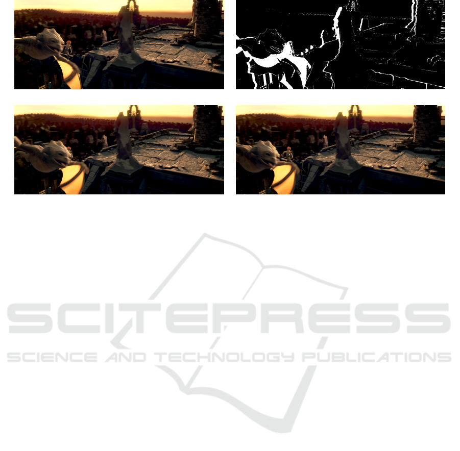
Figure 1: Motivation of the proposed data terms and their dependence on the occlusion map. Notice that most part of the
girl in I
t
l
is not visible in I
t+1
l
while it is visible in I
t+1
r
. Thus, the deactivation of the data term between images I
t
l
and I
t+1
l
together with the activation of the data term relating I
t
l
and I
t+1
r
will result in a better estimation of the scene flow variables.
them estimates the scene flow from RGB-Depth data
benefiting from the availability of depth data provided
by cameras equipped with a depth sensor. The 3D
scene flow is estimated directly from it and regular-
ization of the flow field is imposed on the 3D sur-
faces of the observed scene instead of on the image
plane (Pons et al., 2007; Basha et al., 2013; Jaimez
et al., 2015; Quiroga et al., 2014; Sun et al., 2015;
Vogel et al., 2015). For instance, (Basha et al., 2013;
Vogel et al., 2011) jointly estimate depth and a 3D
flow field using a variational method which imposes
geometric multi-view consistency and 3D smooth-
ness. Some of these methods also use a local rigid-
ity assumption (Menze and Geiger, 2015; Quiroga
et al., 2014) representing the dynamic scene, e.g., as
a collection of rigidly moving planes (Vogel et al.,
2015). The second kind of methods work on stereo
video sequences and estimate from them disparity
(between the stereo pair) and motion (between con-
secutive frames) using formulations which mutually
constrain the scene flow (Huguet and Devernay, 2007;
Wedel et al., 2011). The authors of (Wedel et al.,
2011) propose to precompute the stereo disparity and
decouple depth and motion estimation by estimat-
ing the optical flow and the disparity change through
time.
In most of the proposals, the problem is frequently
modeled by variational methods where the unknowns
representing the motion of each 3D point in the scene
are estimated as the minimum of an energy functional
(e.g., (Vedula et al., 2005; Pons et al., 2007; Huguet
and Devernay, 2007; Basha et al., 2013; Menze and
Geiger, 2015; Wedel et al., 2011)). The optimiza-
tion usually proceeds in a multi-scale or coarse-to-fine
procedure and thus smooth motions are favoured and
large displacements of small objects are mostly lost.
The variational method we propose does not as-
sume a depth sensor is available nor calibrated cam-
eras. As in (Huguet and Devernay, 2007; Wedel
et al., 2011), we use a two-view setup with a pair
of stereo image frames. Our proposal also estimates
motion occlusions and benefits from the appropriate
comparison among views of the scene. In order to
correctly estimate large displacements of small ob-
jects, our minimization works by incorporating sparse
matches which drive the minimization of the energy
in local patches, providing a fast method that works
at the finest scale, i.e., the original scale of the image
data.
3 SCENE FLOW MODEL
Let us assume that a stereo video sequence is given,
consisting of different image pairs that have been ob-
tained from two views. For each time instant t, let
I
t
l
, I
t
r
, I
t+1
l
, I
t+1
r
: Ω → R be two of those consecutive
stereo pair of frames of the stereo video sequence,
where the subscripts l and r stand for left and right,
respectively, and t stands for time. As usual, we as-
sume that the image domain Ω is a rectangle in R
2
.
Our starting point will be the model for scene flow in-
troduced in (Wedel et al., 2011), where a decoupled
approach was presented. In a decoupled approach,
Joint Large Displacement Scene Flow and Occlusion Variational Estimation
173

Figure 2: Diagram with the main steps of the proposed method.
the estimation of depth or disparity at fixed time is
done previously to, and independently of, the estima-
tion of the motion (optical flow and disparity change).
This problem separation provides more flexibility and
has some advantages as the disparity may be esti-
mated with an optimal stereo algorithm. The decou-
pled scene flow approach enforces a coupling among
disparity, optical flow, and disparity change.
Let d be a given disparity map between I
t
l
and I
t
r
.
Let u = (u, v) denote the optical flow between the left
frames, I
t
l
and I
t+1
l
, and δd denote the change in dis-
parity between the stereo pairs at times t and t + 1.
In order to write the energy model in a more compact
form, let us first introduce the following notation:
D
1
= I
t+1
l
(x+u, y+v) −I
t
l
(x, y)
D
2
= I
t+1
l
(x+u, y+v) −I
t
r
(x+d, y)
D
3
= I
t+1
r
(x+d+u+δd, y+v) −I
t+1
l
(x+u, y+v)
D
4
= I
t+1
r
(x+d+u +δd, y+v) −I
t
l
(x, y)
D
5
= I
t+1
r
(x+d+ u+δd, y+v) −I
t
r
(x+d, y)
In order to compute the scene flow field (u, v, δd),
Wedel et al. (Wedel et al., 2011) propose to
minimize an energy functional which is made
of two terms, namely,
¯
E(u, v, δd) =
¯
E
R
(u, v, δd) +
¯
E
D
(u, v, δd), where
¯
E
R
(u, v, δd) = α
Z
Ω
Ψ(|∇u|
2
+|∇v|
2
+γ|∇δd|
2
)dxdy
¯
E
D
(u, v, δd) =
Z
Ω
Ψ(|D
1
|
2
)dxdy
+
Z
Ω
oΨ(|D
3
|
2
)dxdy +
Z
Ω
oΨ(|D
5
|
2
)dxdy
where Ψ(s
2
) =
√
s
2
+ ε
2
, with ε = 0.0001 being a
small constant, and o(x, y, t) is the given stereo visibil-
ity map for the given disparity map d (i.e., o(x, y, t) =
1 if (x, y) is visible both in I
t
l
and in I
t
r
). We have
omitted in
¯
E,
¯
E
R
,
¯
E
D
the dependency of u, v, δd, d, o on
x, y, t for the sake of simplicity. Finally, let us notice
that the regularity term is based on a differentiable ap-
proximation of the Total Variation. Similarly, the data
term is based on the same differentiable approxima-
tion of the L
1
norm of the constraints favoring con-
stancy in intensity of the same point in the scene, thus
in the four involved images.
This method does not directly take occlusions
into account and relies on data terms that consider
correspondence errors even for the occluded pix-
els where no correspondence can be established.
Hence, erroneous flows are generated at moving oc-
clusion boundaries. Explicitly modeling occlusions
has proved beneficial in optical flow estimation meth-
ods (e.g. (Ayvaci et al., 2012; Ballester et al., 2012;
Ince and Konrad, 2008) among others). Occlusion
reasoning has been considered in scene flow estima-
tion methods that use depth sensors (Wang et al.,
2015; Zanfir and Sminchisescu, 2015). On the other
hand, it is traditionally believed that motion vectors
tend to be smaller in magnitude than disparities, espe-
cially if the video sequences have been captured with
a small time delay; but this assumption does not hold
for the current standard databases (Butler et al., 2012;
Geiger et al., 2012) which contain important large dis-
placements. In these situations, handling occlusions
due to motion is as important as handling occlusions
due to disparity.
In this work we extend the previous model to
jointly compute the optical flow, its associated occlu-
sions, and the disparity change. Let χ : Ω → [0, 1] be
the function modeling the motion occlusion map, so
that χ(x , y, t) = 1 identifies the motion occluded pix-
els, i.e. pixels that are visible in I
t
l
but not in I
t+1
l
. Our
model is based on the assumption that the occluded
region due to motion, given by χ(x, y, t) = 1, should
include the region where the divergence of the opti-
cal flow is negative. This was pointed out by Sand
and Teller (Sand and Teller, 2008), who noticed that
the divergence of the motion field may be used to
distinguish between different types of motion areas.
Schematically, the divergence of a flow field is nega-
tive for occluded areas, positive for disoccluded, and
near zero for the matched areas. Taking this into ac-
count, Ballester et al. (Ballester et al., 2012) proposed
a variational model for the joint estimation of occlu-
VISAPP 2017 - International Conference on Computer Vision Theory and Applications
174

sions and optical flow. In order to consider motion
occlusions and benefit from an appropriate compari-
son among the different views of the scene, we build
up from these ideas and propose to include a new term
in the energy functional that characterizes the occlu-
sion areas as those where the divergence of the flow is
negative. We also propose to include different types
of data terms in the energy functional which are acti-
vated based on the occlusion information provided by
χ. In this way, if there is a motion occlusion in the left
view, χ = 1, the energy will only consider error corre-
spondences in the right views, where the object is still
visible. Figure 1 presents an example motivating our
proposal; by detecting the occlusion regions, the mo-
tion field in these regions will be recovered by using
the fact that they are visible in the remaining views
which we use to introduce new data constraints. Thus,
the proposed energy contains three parts, namely,
(1)
E(u, v, δd, χ) = E
R
(u, v, δd, χ) + E
D
(u, v, δd, χ)
+ E
occ
(u, v, χ)
where
E
R
(u, v, δd, χ) = α
Z
Ω
Ψ
|∇u|
2
+|∇v|
2
+γ|∇δd|
2
+ η
Z
Ω
Ψ
|∇χ|
2
E
occ
(u, v, χ) = β
Z
Ω
χdiv(u, v)dx dy
E
D
(u, v, δd, χ) =
Z
Ω
(1 −χ)Ψ(|D
1
|
2
)dxdy
+
Z
Ω
(1 −χ)o Ψ(|D
2
|
2
)dxdy
+
Z
Ω
(1 −χ)o Ψ(|D
3
|
2
)dxdy
+
Z
Ω
χo Ψ(|D
4
|
2
)dxdy
+
Z
Ω
χo Ψ(|D
5
|
2
)dxdy
Again, the map χ is evaluated in (x, y, t) in the func-
tional but we omit it for the ease of notation.
4 OPTIMIZATION STRATEGY
In order to make the optimization problem more
tractable, optical flow variational methods include a
linearization of the warped images in the data terms,
which leads to embed the functional into a coarse-to-
fine multi-level approach to better handle large mo-
tion fields. However, this approach still fails to re-
cover large motions of small objects not present at
coarser scales. Different approaches to overcome
this limitation have been proposed in the past years.
Among the most recent works, several ones share
the trait of being based on a sparse-to-dense estima-
tion that avoids the classical coarse-to-fine scheme.
They start with a set of correspondences (non-dense
feature-based matches), which are used to generate
a dense optical flow field and subsequently, the next
step produces a global refinement over the whole im-
age domain. For instance, in the work (Palomares
et al., 2016), an initial set of sparse matches is grown
by a coordinate descent scheme used to minimize the
target energy functional. Our proposal builds upon
these ideas to propose a minimization method for the
scene flow energy. Figure 2 shows a diagram with the
main steps of the proposed algorithm. The optimiza-
tion process works in two stages, with a previous ini-
tialization of the sparse matches (named as zero stage
in the following), both of them operating at the finest
scale of the image:
0. The zero stage builds the initial set of sparse seeds
(u, v, δd). The algorithm assumes that a set of
sparse correspondences between two pairs of im-
ages are provided; in particular, between I
t
l
↔I
t+1
l
and I
t+1
l
↔I
t+1
r
. In order to estimate sparse corre-
spondences between both pairs of images we use
the DeepMatching algorithm (Weinzaepfel et al.,
2013). From the first set of matchings, between
I
t
l
↔I
t+1
l
, we obtain an initial set of candidates for
the variables (u, v). Then, to completely define the
set of seeds for solving the scene flow problem, it
is necessary to find an estimation of δd(x) asso-
ciated to each optical flow candidate (u(x), v(x))
at the different sparse locations x = (x, y) ∈ Ω.
From the second set of sparse matches, between
I
t+1
l
↔I
t+1
r
, we select the discrete value of
ˆ
d
t+1
to
be the disparity associated of the closest keypoint
ˆ
x in I
t+1
l
(with a matching in I
t+1
r
) to the posi-
tion (x + u(x), y + v(x)) within a certain tolerated
distance. If there exists such a keypoint in I
t+1
l
,
we add (u(x), v(x), δd(x), χ(x)) as an initial seed,
where δd(x) =
ˆ
d
t+1
(
ˆ
x) −d
t
(x) and χ(x) = 0.
1. The first stage consists in computing a dense
scene flow estimation providing a good local min-
imum of the target energy (the proposed (1) in
this paper); good in the sense that captures large
displacements and controls the error on occlu-
sion areas. Our method proceeds by minimiz-
ing the energy over local neighborhoods (patches)
in a proper order defined by the reliability of
the scene flow estimation at the center of each
patch. This ordering is managed by a priority
queue where the most reliable estimations – the
estimated (u, v, δd, χ) values that have the lowest
energy values – are placed at the top positions of
Joint Large Displacement Scene Flow and Occlusion Variational Estimation
175

the queue. Initially, the queue is formed by the
sparse set of seeds. These seeds have an associ-
ated local energy equal to zero (full reliability).
Then, an iterative process is launched; the follow-
ing procedure is iterated until the priority queue is
emptied:
• The top element of the queue of scene flow
candidates is extracted and its associated scene
flow value is set as visited at its corresponding
position.
• The patch around the visited position is consid-
ered and a scene flow is interpolated within the
patch by propagating the already visited values.
• The scene flow energy is minimized in the
patch, starting with the previous interpolation
as initialization. Notice that this step can be
thought as a minimization of the energy where
all the variables outside the patch under con-
sideration have been fixed, thus bearing simi-
larities with the coordinate descent methods.
• The local energy in the patch is computed and
the four immediate neighbors of the center
pixel are introduced as new candidates in the
queue with a reliability given by the local en-
ergy (the energy of the patch).
2. The result of the first step, the data correspond-
ing to (u, v, δd, χ), is a dense scene flow estima-
tion providing a good local minimum of the en-
ergy (1).This result is refined in the second stage
by the minimization of the energy functional over
the whole image domain. In other words, the re-
sult of the first step is used as an initialization for
minimizing the energy around it.
Let us remark that the method of Cech et al. (Cech
et al., 2011) also uses an algorithm to estimate both
disparity and optical flow from a stereo sequence by
growing a set of seeds. In contrast to our seed grow-
ing method driven by the energy minimization, the
method in (Cech et al., 2011) constructs heuristics
based on photometric consistency through correla-
tions and constant parameters adjusting the amount of
optical flow regularization and temporal consistency.
Moreover, it provides a semi-dense scene flow while
we get a dense estimation.
In order to minimize our energy formulation (1),
the associated Euler-Lagrange equations are numeri-
cally solved. To simplify the presentation, we intro-
duce the following notations
R
m
=
q
|∇u|
2
+|∇v|
2
+γ|∇δd|
2
R
o
= |∇χ|
Ψ
0
(s
2
) =
1
2
√
s
2
+ ε
2
Thereby, the Euler-Lagrange equations are
0 = −α div
Ψ
0
(R
2
m
) ·∇u
+ (1 −χ) ·Ψ
0
(D
2
1
) ·D
1
·I
t+1
l,x
(x+u, y+v)
+ o (1 −χ) ·Ψ
0
(D
2
2
) ·D
2
·I
t+1
l,x
(x+u, y+v)
+ o (1 −χ) ·Ψ
0
(D
2
3
) ·D
3
·(I
t+1
r,x
(x+d+u+δd, y+v)
−I
t+1
l,x
(x+u, y+v))
+ o χ ·Ψ
0
(D
2
4
) ·D
4
·I
t+1
r,x
(x+d+u+δd, y+v)
+ o χ ·Ψ
0
(D
2
5
) ·D
5
·I
t+1
r,x
(x+d+u+δd, y+v)
−βχ
x
,
0 = −α div
Ψ
0
(R
2
m
) ·∇v
+ (1 −χ) ·Ψ
0
(D
2
1
) ·D
1
·I
t+1
l,y
(x+u, y+v)
+ o (1 −χ) ·Ψ
0
(D
2
2
) ·D
2
·I
t+1
l,y
(x+u, y+v)
+ o (1 −χ) ·Ψ
0
(D
2
3
) ·D
3
·(I
t+1
r,x
(y+d+u+δd, y+v)
−I
t+1
l,y
(x+u, y+v))
+ o χ ·Ψ
0
(D
2
4
) ·D
4
·I
t+1
r,y
(x+d+u+δd, y+v)
+ o χ ·Ψ
0
(D
2
5
) ·D
5
·I
t+1
r,y
(x+d+u+δd, y+v)
− βχ
y
,
0 = −αγ div
Ψ
0
(R
2
m
) ·∇δd
+ o (1 −χ)Ψ
0
(D
2
3
) ·D
3
·I
t+1
r,x
(x+d+u+δd, y+v)
+ o χ ·Ψ
0
(D
2
4
) ·D
4
·I
t+1
r,x
(x+d+u+δd, y+v)
+ o χ ·Ψ
0
(D
2
5
) ·D
5
·I
t+1
r,x
(x+d+u+δd, y+v) ,
0 = −αη div
Ψ
0
(R
2
o
) ·∇χ
− Ψ(D
2
1
) −Ψ(D
2
2
) −o
Ψ(D
2
3
) + Ψ(D
2
4
) + Ψ(D
2
5
)
+ βdiv(u, v) .
where the subindices x and y denote the partial
derivatives with respect to x and y, respectively, and
the point coordinates (x, y) have been omitted in the
gradient expressions.
The Euler-Lagrange equations are non-linear in
the unknowns (u, v, δd, χ) due to the multiple warped
images I
t+1
l
(x+u, y+v), I
t+1
l,x
(x+u, y+v), etc. To nu-
merically solve them, either over a local patch or over
the whole domain, we follow the optimization method
proposed by Brox et al. (Brox et al., 2004). It is based
on two fixed iterations loops to cope with the non-
linear terms. The external loop is used to handle the
linearization of the data terms in the warped form, and
the internal loop takes into account the non-linearities
of the Ψ
0
functions. After the linearization, the result-
ing linear system can be efficiently solved using the
SOR method (Young, 1971).
VISAPP 2017 - International Conference on Computer Vision Theory and Applications
176

Example 1: First frame Coarse-to-fine minimization Ground truth Proposed minimization
Example 2: First frame Coarse-to-fine minimization Ground truth Proposed minimization
Example 3: First frame Coarse-to-fine minimization Ground truth Proposed minimization
Figure 3: Comparison of two minimization strategies for the same energy proposed in (Wedel et al., 2011). Our minimization
startegy is not based on a coarse-to-fine scheme but on sparse correspondences that allow to capture large displacements.
Results in the MPI Sintel training set.
5 EXPERIMENTS
In this section we provide two sets of experiments.
The first one is designed to validate the better be-
haviour of the selected optimization strategy against
the classic coarse-to-fine multi-level approach. The
second one shows the properties of the presented
functional due to the explicitly occlusion handling.
Let us remark that all results have been obtained
by using the grayscale versions of the original color
frames. The color version is only used to compute
the seeds with the Deep Matching algorithm. The ex-
periments use stereo sequences from the MPI Sintel
Flow dataset (Butler et al., 2012) and from the KITTI
2015 dataset (Menze and Geiger, 2015). Sintel has
23 training sequences. For every frame, there are two
different versions of the images, “clean” and “final”.
The difference is that the second set adds complexity
to the first one by incorporating atmospheric effects,
depth of field blur, motion blur, color correction and
other details. It contains several sequences with large
motions of small objects. KITTI contains different
sequences of a city provided by an autonomous driv-
ing platform. It presents large deformations, dynamic
scenes and challenging iluminatons changes.
5.1 Benefits of the New Optimization
Strategy
Our first goal is to validate the good performance of
the optimization scheme and show the benefits in the
presence of large displacement motions against the
coarse-to-fine strategy. For this purpose, we use the
energy functional proposed by Wedel et al. (Wedel
et al., 2011) (detailed at the beginning of Section 3),
and we compute the motion field using these two dif-
ferent minimization approaches. In Tables 1 and 2,
they are denoted by Classic Wedel (i.e., classic coarse-
to-fine strategy for the Wedel et al. (Wedel et al.,
2011) energy) and Our Wedel. Fig. 3, Tables 1 and 2
show that the chosen minimization approach is able to
recover large motions where the coarse-to-fine strat-
egy fails. For each group of four images in Fig. 3,
from top to bottom and from left to right, the first
frame is displayed in (a), the optical flow estimation
from the classic coarse-to-fine Wedel et al. (Wedel
et al., 2011) is displayed in (b), (c) shows the opti-
cal flow ground truth, and (d) the optical flow esti-
mated with our scene flow minimization strategy for
the same energy. Let us notice from this figure and
also from Tables 1 and 2 that the optimization scheme
is also better for the kind of sequences where the
multi-scale approach does not fail. It is clear that the
integration of sparse matches results with an appropri-
ate minimization strategy directly at the finest image
scale represents a great improvement in comparison
to the coarse-to-fine optimization strategy.
5.2 Benefits of the New Energy
The second goal is to show the advantages of the
proposed energy functional which includes new data
terms and motion occlusion estimation. Fig. 4 dis-
plays results on three sequences of the MPI Sintel
training set. For each group of six images, from top to
bottom and from left to right, the first frame is shown
in (a), the ground truth occlusions are displayed in
(b), (c) shows the optical flow from our scene flow
minimization strategy for the Wedel et al. (Wedel
et al., 2011) energy (our Wedel), (d) the optical flow
ground truth, and (e) and (f) the occlusions and opti-
Joint Large Displacement Scene Flow and Occlusion Variational Estimation
177
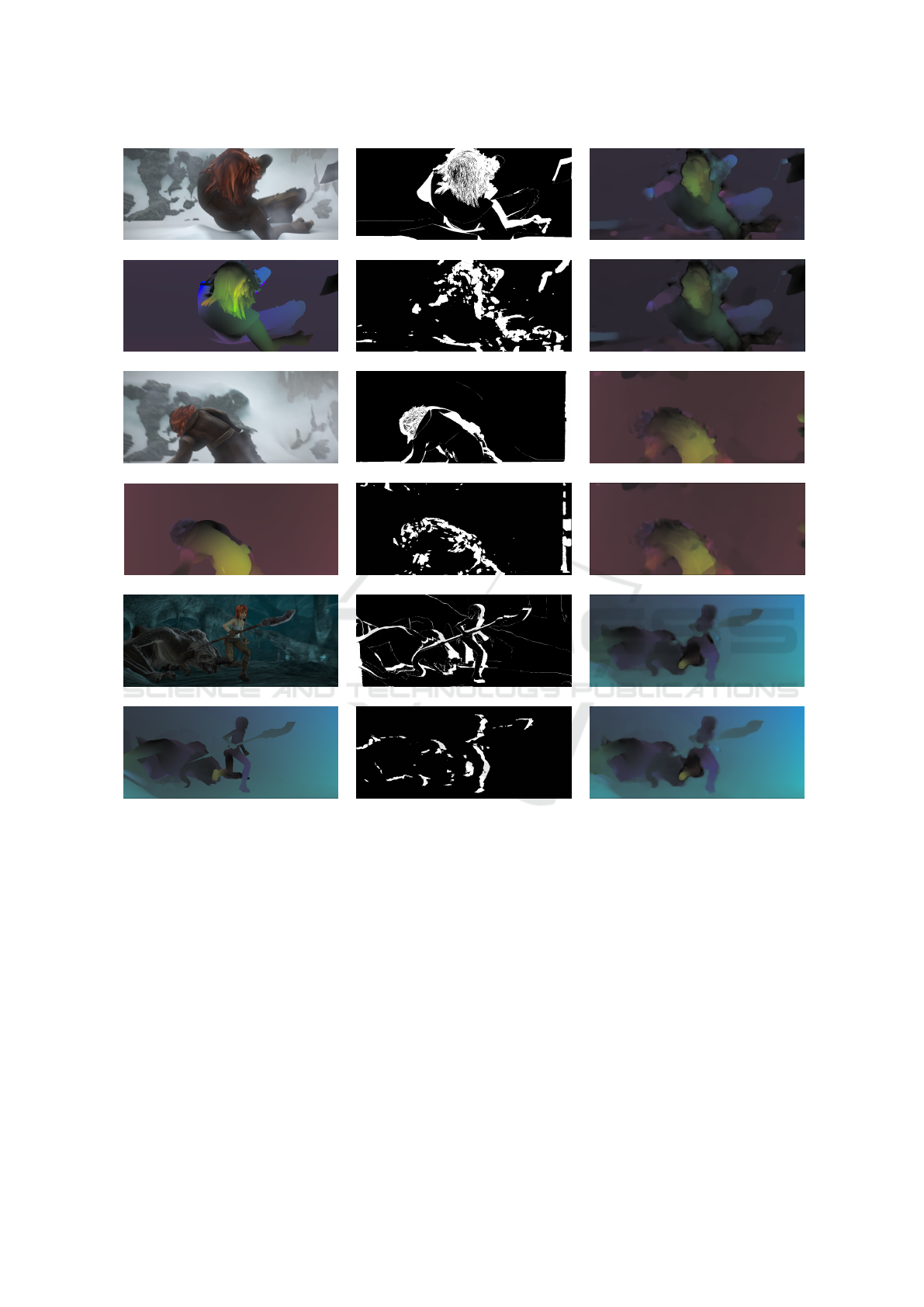
Example 1: First frame Ground truth occlusions OF with energy (Wedel et al., 2011)
OF ground truth Estimated occlusions OF with our energy (1)
Example 2: First frame Ground truth occlusions OF with energy (Wedel et al., 2011)
OF ground truth Estimated occlusions OF with our energy (1)
Example 3: First frame Ground truth occlusions OF with energy (Wedel et al., 2011)
OF ground truth Estimated occlusions OF with our energy (1)
Figure 4: Comparison of the estimated optical flows (OF) estimated with the baseline energy (Wedel et al., 2011) and with
the new proposed energy (1) (in both cases using our proposed minimization strategy). Results in the MPI Sintel training set.
cal flow estimated from our whole proposal with the
energy (1). On the other hand, the second and third
rows of Table 1 and Table 2 show the global accu-
racy over the whole datasets of both proposals. The
results of Table 1 and Fig. 4, show that the proposed
energy keeps better results at the visible areas (sec-
ond column of Table 1) and it specially improves the
accuracy at the occluded areas (third column). The
occlusion mask allows to densely reinforce the 3D ge-
ometry from the fact that points that are occluded in
time in the left view might be visible from the other
(right) view and thus obtain better optical flow bound-
aries especially near occlusion regions. This effect is
noticeable for instance in the boundaries of the nagi-
nata in the experiment of the last rows of Fig. 4.
6 CONCLUSIONS
We have proposed a variational model for the joint
estimation of the scene flow and its associated motion
occlusions. Our work stems from the classical scene
flow model presented in (Wedel et al., 2011) and in-
corporates a characterization of the occlusion areas as
well as new data terms. The estimation of the oc-
clusion map is useful to select a different set of data
VISAPP 2017 - International Conference on Computer Vision Theory and Applications
178

Table 1: Results in MPI-Sintel training set for the optical
flow (u, v) and for the disparity change δd. The first and
second set of results correspond, respectively, to the Final
and Clean frames. EPE means endpoint error over the com-
plete frames. EPE-M shows the endpoint error over regions
that remain visible in adjacent frames. EPE-U shows the
endpoint error over regions that are visible only in one of
the two adjacent frames. Notice that the ground truth δd
is not provided in the database. We have set δd(x, y) =
δd
t+1
(x + u, y + v) −d(x, y) using the (u, v, d
t
, d
t+1
) ground
truth values. Using that information we have obtained the
EPE-δd for all the image.
EPE EPE-M EPE-U EPE-δd
Final
Classic Wedel 9.1461 7.7189 17.7888 1.1234
Our Wedel 7.6287 5.3934 19.8561 0.8121
Our Proposal 7.5095 5.2406 18.9948 0.7997
Clean
Classic Wedel 8.6722 7.2324 17.2608 1.03522
Our Wedel 4.5097 2.2905 15.5042 0.5634
Our Proposal 4.3041 2.1558 15.1603 0.5521
Table 2: Results in KITTI 2015 training dataset for the op-
tical flow (u, v) and for the disparity change δd. Out-noc
(resp. Out-all) refers to the percentage of pixels where the
estimated optical flow presents an error above 3 pixels in
non-occluded areas (resp. all pixels). Out-δd refers to the
percentage of pixels where the estimated disparity change
presents an error above 3 pixels in the pixels where the dis-
parity is available.
Out-noc Out-all Out-δd
Classic Wedel 45.8745 55.4356 42.8971
Our Wedel 24.4237 33.2209 31.8971
Our Proposal 23.5233 32.8576 30.7532
terms for the occluded pixels, i.e., data terms that de-
pend on the views where these pixels might be visible.
We also have extended the optimization method for
optical flow problems presented in (Palomares et al.,
2016) to the scene flow case. Experimental results
show, both quantitative and qualitatively, the benefits
of the proposed energy functional and the minimiza-
tion strategy. As future work we plan to use regular-
ization and data terms that better preserve the image
boundaries and that are more robust to illumination
changes.
ACKNOWLEDGEMENTS
The authors acknowledge partial support by
TIN2015-70410-C2-1-R (MINECO/FEDER, UE)
and by GRC reference 2014 SGR 1301, Generalitat
de Catalunya.
REFERENCES
Ayvaci, A., Raptis, M., and Soatto, S. (2012). Sparse occlu-
sion detection with optical flow. International Journal
of Computer Vision, 97(3):322–338.
Ballester, C., Garrido, L., Lazcano, V., and Caselles, V.
(2012). A tv-l1 optical flow method with occlusion de-
tection. In Pinz, A., Pock, T., Bischof, H., and Leberl,
F., editors, DAGM/OAGM Symposium, volume 7476
of Lecture Notes in Computer Science, pages 31–40.
Springer.
Basha, T., Moses, Y., and Kiryati, N. (2013). Multi-view
scene flow estimation: A view centered variational
approach. International Journal of Computer Vision,
101(1):6–21.
Brox, T., Bruhn, A., Papenberg, N., and Weickert, J. (2004).
High accuracy optical flow estimation based on a the-
ory for warping. In European Conference on Com-
puter Vision (ECCV), volume 3024 of Lecture Notes
in Computer Science, pages 25–36. Springer.
Butler, D. J., Wulff, J., Stanley, G. B., and Black, M. J.
(2012). A naturalistic open source movie for optical
flow evaluation. In European Conference on Com-
puter Vision, pages 611–625.
Cech, J., Sanchez-Riera, J., and Horaud, R. P. (2011). Scene
flow estimation by growing correspondence seeds. In
Proceedings of the IEEE Conference on Computer Vi-
sion and Pattern Recognition, pages 3129–3136.
Geiger, A., Lenz, P., and Urtasun, R. (2012). Are we ready
for autonomous driving? the kitti vision benchmark
suite. In Conference on Computer Vision and Pattern
Recognition (CVPR).
Huguet, F. and Devernay, F. (2007). A variational method
for scene flow estimation from stereo sequences. In
Computer Vision, 2007. ICCV 2007. IEEE 11th Inter-
national Conference on, pages 1–7.
Ince, S. and Konrad, J. (2008). Occlusion-aware optical
flow estimation. IEEE Transactions on Image Process-
ing, 17(8):1443–1451.
Jaimez, M., Souiai, M., Stueckler, J., Gonzalez-Jimenez,
J., and Cremers, D. (2015). Motion coopera-
tion: Smooth piece-wise rigid scene flow from rgb-
d images. In Proc. of the Int. Conference on
3D Vision (3DV). ¡a href=”https://youtu.be/qjPsKb-
˙kvE”target=”˙blank”¿[video]¡/a¿.
Menze, M. and Geiger, A. (2015). Object scene flow for au-
tonomous vehicles. In The IEEE Conference on Com-
puter Vision and Pattern Recognition (CVPR).
Palomares, R. P., Meinhardt-Llopis, E., Ballester, C., and
Haro, G. (2016). Faldoi: A new minimization strategy
for large displacement variational optical flow. Journal
of Mathematical Imaging and Vision, pages 1–20.
Pons, J. P., Keriven, R., and Faugeras, O. (2007). Multi-
view stereo reconstruction and scene flow estimation
Joint Large Displacement Scene Flow and Occlusion Variational Estimation
179

with a global image-based matching score. Interna-
tional Journal on Computer Vision, 72(2):179–193.
Quiroga, J., Brox, T., Devernay, F., and Crowley, J. (2014).
Dense semi-rigid scene flow estimation from rgbd im-
ages. In ECCV 2014, pages 567–582.
Sand, P. and Teller, S. (2008). Particle video: Long-range
motion estimation using point trajectories. Interna-
tional Journal of Computer Vision, 80(1):72–91.
Sun, D., Sudderth, E. B., and Pfister, H. (2015). Layered
rgbd scene flow estimation. In Computer Vision and
Pattern Recognition (CVPR), 2015 IEEE Conference
on, pages 548–556.
Vedula, S. and et al. (1999). Three-dimensional scene flow.
In Computer Vision, 1999. The Proceedings of the
Seventh IEEE International Conference on. IEEE, vol-
ume 2, pages 722–729.
Vedula, S., Rander, P., Collins, R., and Kanade, T.
(2005). Three-dimensional scene flow. Pattern Anal-
ysis and Machine Intelligence, IEEE Transactions on,
27(3):475–480.
Vogel, C., Schindler, K., and Roth, S. (2011). 3d scene
flow estimation with a rigid motion prior. In Computer
Vision (ICCV), 2011 IEEE International Conference
on, pages 1291–1298.
Vogel, C., Schindler, K., and Roth, S. (2015). 3d scene
flow estimation with a piecewise rigid scene model.
International Journal of Computer Vision, 115(1):1–
28.
Wang, Y., Zhang, J., Liu, Z., Wu, Q., Chou, P. A., Zhang,
Z., and Jia, Y. (2015). Handling occlusion and large
displacement through improved rgb-d scene flow esti-
mation. IEEE Transactions on Circuits and Systems
for Video Technology, 26(7):1265–1278.
Wedel, A., Brox, T., Vaudrey, T., Rabe, C., Franke, U., and
Cremers, D. (2011). Stereoscopic scene flow com-
putation for 3d motion understanding. International
Journal of Computer Vision, 95(1):29–51.
Weinzaepfel, P., Revaud, J., Harchaoui, Z., and Schmid,
C. (2013). DeepFlow : Large displacement optical
flow with deep matching. International Conference
on Computer Vision.
Young, D. M. (1971). Iterative solution of large linear sys-
tems. Computer science and applied mathematics.
Academic Press, Orlando.
Zanfir, A. and Sminchisescu, C. (2015). Large displacement
3d scene flow with occlusion reasoning. In Proceed-
ings of the IEEE International Conference on Com-
puter Vision, pages 4417–4425.
VISAPP 2017 - International Conference on Computer Vision Theory and Applications
180
