Robust Gain-scheduling LPV Control for a Reconﬁgurable Robot

R. Al Saidi

and S. Alirezaee

University of Windsor, Windsor, Canada

Electrical and Computer Engineering Department, Windsor, Canada

Keywords:

Reconﬁgurable Robot, Variable D-H Parameters, Gain-scheduling Control, LPV Control.

Abstract:

This paper develops a robust gain–scheduling linear parameter varying (LPV) control for a reconﬁgurable

robot that combines as many properties of different open kinematic structures as possible and can be used for

a variety of applications. The kinematic design parameters, i.e., the Denavit–Hartenberg (D–H) parameters,

can be modiﬁed to satisfy any conﬁguration required to meet a speciﬁc task. By varying the joint twist angle

parameter (a conﬁguration parameter), the presented model is reconﬁgurable to any desired open kinematic

structure, such as ABB, FANUC and SCARA robotic systems. A robust LPV control is developed for on–line

measured parameters of a perturbed LPV model of a Bosch Scara robot arm. This control achieves superior

tracking performance in the presence of dynamic and parameter uncertainties.

1 INTRODUCTION

Robotics technology has been recently exploited in

a variety of areas and various robots have been de-

veloped to accomplish sophisticated tasks in differ-

ent ﬁelds and applications such as in space explo-

ration, future manufacturing systems, medical tech-

nology, etc. In space, robots are expected to complete

different tasks, such as capturing a target, construct-

ing a large structure and autonomously maintaining

in-orbit systems. The rapid changes and adjustments

of the Reconﬁgurable Manufacturing Systems (RMS)

structure must happen in a relatively short time rang-

ing between minutes and hours and not days or weeks.

These systems’ reconﬁgurability calls for their com-

ponents, such as machines and robots to be rapidly

and efﬁciently modiﬁable to varying demands. In

these missions, one fundamental task with the robot

would be the tracking of changing workspace, paths,

the grasping and the positioning of a target in Carte-

sian space. It is desirable and cost effective to em-

ploy a single versatile robot capable of performing

tasks such as inspection, contact operations, assem-

bly (insertion or removal parts), and carrying ob-

jects (pick and place). To satisfy such varying envi-

ronments, a robot with changeable (kinematic struc-

ture) conﬁguration is necessary to cope with these

requirements and tasks. In the literature, LPV con-

trol is used for predeﬁned (ﬁxed) kinematic struc-

ture robots achieving speciﬁc tracking performance

requirements. Methodologies for designing LPV con-

trol are given in (Packard, 1994), (Apkarian and

Adams, 1997), (P. Gahinet, 1994) and (Kemin Zhou,

1996), where the gain scheduled controller was guar-

anteed for H

∞

performance of a class of LPV non-

linear systems. In (Zhongwei Yu, 2003) and (Seyed

Mahdi Hashemi, 2009) a polytopic gain scheduled H

∞

control is developed for a two Degrees Of Freedom

(DOF) robot considering nominal parameters without

uncertainties. In (Y.Sun and Liang, 2018), an LPV

controller is developed for a large number of afﬁne

scheduling dynamic parameters of a 2 DOF robot ma-

nipulator without considering uncertainties in their

robotic model.

2 KINEMATICS DEVELOPMENT

OF A RECONFIGURABLE

ROBOT

Development of the general n–DOF Global Kine-

matic Model (n–GKM) is necessary for supporting

any open kinematic robotic arm. The n–GKM model

is generated by the variable D–H parameters as pro-

posed in (A. Djuric, 2010). The D–H parameters pre-

sented in Table 1 are modeled as variable parameters

to accommodate all possible open kinematic struc-

tures of a robotic arm. The twist angle variable α

is limited to ﬁve different values, (0

,±90

,±180

Al Saidi, R. and Alirezaee, S.

Robust Gain-scheduling LPV Control for a Reconﬁgurable Robot.

DOI: 10.5220/0011356000003271

In Proceedings of the 19th International Conference on Informatics in Control, Automation and Robotics (ICINCO 2022), pages 89-96

ISBN: 978-989-758-585-2; ISSN: 2184-2809

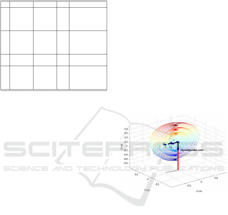
Table 1: D–H parameters of the n-GKM model.

i d

DH1

,±180

,±90

DH1

DH2

,±180

,±90

DH2

. . .

. . . . . . . . . . . .

DHn

,±180

,±90

DHn

The subscript DHn implies that the d

or θ

parameter is

constant.

to maintain perpendicularity between joints’ coordi-

nate frames. Consequently, each joint has six distinct

positive directions of rotation and/or translation. The

reconﬁgurable joint is a hybrid joint that can be con-

ﬁgured to be either revolute or prismatic type of mo-

tion, according to the required task. For the n–GKM

model, a given joint’s vector z

i−1

can be placed in the

positive or negative directions of the x,y, and z axis in

the Cartesian coordinate frame. This is expressed in

(1) and (2):

Rotational Joints : R

= 1 and T

= 0 (1)

Translational Joints : R

= 0 and T

= 1 (2)

The variables R

and T

are used to control the selec-

tion of joint type (rotational and/or translational). The

orthogonality between the joint’s coordinate frames is

achieved by assigning appropriate values to the twist

angles α

. Their trigonometric functions are deﬁned

as the joint’s reconﬁgurable parameters (K

& K

)

and expressed in (3) and (4):

= sin(α

) (3)

= cos(α

) (4)

The kinematics of a reconﬁgurable robot are calcu-

lated by multiplication of the all homogeneous ma-

trices from the base frame to the ﬂange frame. The

resulting homogeneous transformation matrix for the

(n-GKM) model is given in (5):

i−1







cos(R

+ T

DHi

) −K

sin(R

+ T

DHi

)

sin(R

+ T

DHi

) K

cos(R

+ T

DHi

)

0 K

0 0

(5)

sin(R

+ T

DHi

) a

cos(R

+ T

DHi

)

−K

cos(R

+ T

DHi

) a

sin(R

+ T

DHi

)

DHi

+ T

0 1







i = 1, 2,...,n

The workspace of a reconﬁgurable robot manip-

ulator with similar kinematic structure to the PUMA

560 is calculated and shown in Fig. 1. The resulting

workspace shows a union of three layers which in-

dicates the workspace variability property of any re-

conﬁgurable manipulator. The three workspace lay-

ers are calculated based on turning the third joint into

a prismatic one (transnational motion). The variable

workspace shown in Fig.1 was generated when the

third joint has translated with 0.1, 0.2, 0.3 m.

Figure 1: The workspace of a reconﬁgurable manipulator.

3 DYNAMIC PARAMETER

PROPERTIES OF A

RECONFIGURABLE ROBOT

The equation of motion of a reconﬁgurable robot can

be described with a set of coupled differential equa-

tions in matrix form:

τ = M(q) ¨q +C(q, ˙q) + F ˙q + G(q) (6)

where q, ˙q and ¨q are respectively the vectors of gener-

alized joint coordinates, velocities and accelerations.

M(q) is the joint–space inertia matrix, C(q, ˙q) is the

Coriolis and centripetal coupling matrix, F is the fric-

tion force, G(q) is the gravity loading, and τ is the

vector of generalized actuator torques associated with

the generalized coordinates q. The effect of varying

ICINCO 2022 - 19th International Conference on Informatics in Control, Automation and Robotics

the conﬁgurations of the dynamic parameters such as

gravity and inertia are analyzed for the shoulder and

elbow joints below.

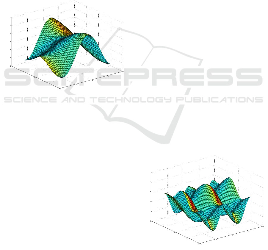
3.1 Gravity Load Parameter

The gravity load term in (6) is generally a dominant

term and present even when the manipulator is sta-

tionary or moving slowly. The torque on a joint due

to gravity acting on the robot depends strongly on the

robot’s pose. The torque on the shoulder joint (q

) is

much greater when the robot is stretched out horizon-

tally as shown in Fig.2, which indicates the relation

between the gravity torque, shoulder (q

) and elbow

) joints.

−4

−2

−4

−2

−30

−20

−10

q2 (rad)

q3 (rad)

g2 (Nm)

Figure 2: Gravity torque variation due to a different conﬁg-

uration pose (shoulder gravity load).

3.2 Inertia Matrix Parameter

The inertia matrix is a positive deﬁnite symmetric ma-

trix in which the matrix elements are functions of the

manipulator pose. The inertia matrix has diagonal el-

ements M

i j

that describe the inertia exerting the joint j

by torque τ

= M

i j

. The ﬁrst two diagonal elements,

corresponding to the robot’s waist and shoulder joints,

are large since motion of these joints involves rotation

of the heavy upper– and lower–arm links. The off-

diagonal terms M

i j

= M

, i ̸= j represent coupling of

acceleration from joint j to the torques and forces on

joint j − 1. The variation of the inertia elements as

a function of robot conﬁgurations are shown in Fig.3.

The results indicate a signiﬁcant variation in the value

of M

which changes by a factor of: max(M

(:)) /

min(M

(:)) = 1.7683. The off–diagonal represents

coupling between the angular acceleration of joint 2

and the torque on joint 1.

4 SYNTHESIS OF

GAIN-SCHEDULED

CONTROLLER

It has been shown from the analysis above that, the

dynamic parameters of a reconﬁgurable robot are

strongly dependent on robot conﬁgurations. These

variable parameters completely deﬁne the operating

point of the robot and are assumed to be measured in

real time. This motivates the design of a control sys-

tem that is scheduled with the measured parameters

such as M(q) and F( ˙q) to provide higher performance

for large variation in these parameters. Gain schedul-

ing or LPV techniques are used for controlling LPV

systems. An LPV controller consists of designing

a linear time invariant (LTI) controller that is adapt-

ing itself when the operating conditions change. In

this control method, the system is assumed to depend

afﬁnely on a measured vector of time varying param-

eters. Assuming on–line measurements of these pa-

rameters, they can be fed to the controller to optimize

the performance and robustness of the closed loop

system.

4.1 Synthesis of LPV Polytopic

Controllers

LPV control is applicable to time varying and non-

linear systems whose linearized dynamics are approx-

imated by an afﬁne parameter dependent system in the

form of:

˙x =A(θ(t))x + B

(θ(t))w + B

(θ(t))u

z =C

(θ(t))x + D

(θ(t))w + D

(θ(t))u

y =C

(θ(t))x + D

(θ(t))w + D

(θ(t))u (7)

where the time varying parameter vector θ(t) ranges

within a known interval. The system (7) is further

−4

−2

−4

−2

2.5

3.5

4.5

q2 (rad)

q3 (rad)

M11 (Kg m

)

Figure 3: Variation of inertia matrix elements M

with con-

ﬁguration.

Robust Gain-scheduling LPV Control for a Reconﬁgurable Robot

assumed to be polytopic:





A(θ(t)) B

(θ(t)) B

(θ(t))

(θ(t)) D

(θ(t))

(θ(t)) D

(θ(t))





∈ Co









11i

12i

21i

22i





,i = 1,2,··· , r





(8)

where A

,··· , denote the values of

A(θ(t)), B

(θ(t)), · · · , at the polytope vertices.

The system matrix dimensions are given by:

A(θ(t)) ∈ R

n×n

(θ(t)) ∈ R

×m

(θ(t)) ∈ R

×m

(9)

An LPV system has a quadratic H

∞

performance γ if

and only if there exists a single positive deﬁnite ma-

trix X > 0 such that:





A(θ(t))

X + XA(θ(t)) XB(θ(t)) C(θ(t))

B(θ(t))

X −γI D(θ(t))

C(θ(t)) D(θ(t)) −γI





< 0

(10)

for all admissible values of the parameter vector θ(t).

An LPV polytopic controller with the same parameter

dependence as the system is given as:

˙x

(θ(t))x + B

(θ(t))w

z =C

(θ(t))x + D

(θ(t))w (11)

Then, the LPV controller (11) can be employed to as-

sure the quadratic H

∞

performance γ of the resulting

closed loop system:

˙x

(θ(t))x + B

(θ(t))w

z =C

(θ(t))x + D

(θ(t))w (12)

where

(θ(t)) =



A(θ(t))+ B

(θ(t))D

(θ(t))C

(θ(t))

(θ(t))C

(θ(t))

(θ(t))C

(θ(t))



(θ(t)) =



(θ(t))+ B

(θ(t))D

(θ(t))

(θ(t))D

(θ(t))



(θ(t)) =



(θ(t))+ D

(θ(t))D

(θ(t))C

(θ(t))

(θ(t))C

(θ(t))



(θ(t)) = D

(θ(t))+ D

(θ(t))D

(θ(t))

(13)

Synthesis of an LPV control is to ensure the follow-

ing:

• The resulting polytopic closed loop system (12)

is enforced to be stable over the entire parameter

polytope and for arbitrary parameter variations.

• The L

–induced norm of the performance sig-

nals are bounded by γ for all possible trajectories

within the parameter vector θ(t).

4.2 Application of LPV Polytopic

Control

A Bosch Scara robot with RRT kinematic structure

is considered where the ﬁrst two joints and links are

shown in Fig.4 (above). The third joint is considered

to be mechanically decoupled from the motions of the

other joints. The inertia and Coriolis matrices are de-

rived as follows:

M(θ) =



+ 2I

cos(θ

) I

+ I

cos(θ

)

+ I

cos(θ

) I



(14)

C(θ,

θ) =

−2I

sin(θ

)

− I

sin(θ

)

sin(θ

)

(15)

The complete system model of the ﬁrst two links

is shown in Fig.4 (below), including servo motors,

and the dynamic cross–coupling torques (Coriolis ef-

fects). A spring–damper is introduced to model the

torsion stiffness of the robot shaft between each DC

motor and the link. The dynamic coupling appears

in the joint systems as torques on the joint axes and is

considered as an independent disturbance torque. The

nominal values of the robot parameters are estimated

at the zero position of the ﬁrst two joints. The state

equations of the ﬁrst link are derived as follows:

˙x

= x

˙x

+ D

− F

+ τ

)

˙x

= N

− x

˙x

− N

− F

)

˙x

(−R

− K

+ x

+ K

p12

u − K

p12

)

˙x

= −k

i12

+ k

i12

y = x

(16)

The derivations of the state equations for the sec-

ond link are omitted for brevity but are similar to the

derivations above.

4.3 Application of LPV Control

In this subsection, an LPV polytopic control is de-

signed for the LPV linear system given in (16)

with two parameters conﬁguration dependent M(q)

and F( ˙q). These two coefﬁcients, satisfy M(q) ∈

min

max

] and F( ˙q) ∈[F

min

max

]. Assuming that

M(q) and F( ˙q) are on–line measurable parameters,

the controller is allowed to incorporate these mea-

surements in the same fashion as the system. The re-

sulting LPV controller exploits all the available mea-

surements of M(q) and F( ˙q) to provide a smooth and

ICINCO 2022 - 19th International Conference on Informatics in Control, Automation and Robotics

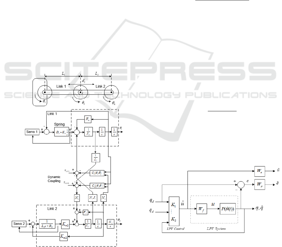
automatic gain scheduling. The LPV control struc-

ture displayed in Fig.5 consists of the LPV linear

system P(θ(t)) and three LPV polytopic controllers.

The reference velocity ˙q

and position q

are fed di-

rectly to the LPV feedforward controllers K

(θ(t))

and K

(θ(t)), respectively, while the robot conﬁgura-

tion position q is fed back to the LPV feedback con-

troller K

(θ(t)). The LTI performance function W

chosen to weight the resulting error e between the ref-

erence position q

and measured joint angle position

q. The function K

(θ(t))S(θ(t)) is weighted using an

LTI input weighting function W

to ensure robustness

against unmodeled dynamics. The LPV control ob-

jectives are as follows:

1. To get internal stability of the closed loop system.

2. To enforce the performance and robustness re-

quirements by minimizing the L

–gain of the

closed loop performance channel.

These objectives should be satisﬁed for the time vary-

ing trajectories M(q) and F( ˙q). The design proce-

dure is performed with describing the LPV system

P(θ(t)) (16) by two afﬁne parameter–dependent mod-

els. Using the LPV loop shaping procedure, the

resulting LPV polytopic system is placed within a

polytope convex hull of four vertex systems Co{P

Figure 4: Schematic top view of the Bosch Scara robot in

zero position (above). Model of ﬁrst two links and servo

motors of the Bosch Scara robot (below).

i = 1,··· , 4}. The vertices P

are the values of P(θ(t))

at the four vertices (the four corners P

,··· , P

) of the

following parameter box:



max



, p



min

max





max

min



, p



min



(17)

The LPV synthesis problem illustrated in Fig.5 is

solved using the Matlab/Linear Matrix Inequality

(LMI) control toolbox. To solve this problem, the in-

put should be parameter independent (Apkarian and

Adams, 1997). This condition is satisﬁed by pre–

ﬁltering the control input u with a high pass ﬁlter W

as follows:

(s + 2π ∗ 100 ∗ 0.4)

(1/2000s + 2π ∗ 100)

(18)

The optimization problem is to ﬁnd an LPV controller

to minimize:



(19)

The performance weighting functions W

and W

are

designed to enforce the performance and robustness

speciﬁcations in (19). An appropriate scaling of the

system has been performed so that the input is less

than or equal to one in magnitude, and therefore a

simple input weight W

= 1 is selected. The perfor-

mance weight is chosen as follows:

(s/M + w

)

s + w

(20)

The value w

= 10 has been selected to achieve ap-

proximately the desired crossover frequency w

of 10

rad/s. The steady state error requirement is deter-

mined by the selection of the parameter value of A,

which is chosen to be A = 10

−4

Figure 5: LPV control structure includes the LPV

system P(θ(t)), performance weighting function W

robustness function W

, LPV polytopic controllers

(θ(t)),··· ,K

(θ(t)) and input ﬁlter W

Robust Gain-scheduling LPV Control for a Reconﬁgurable Robot

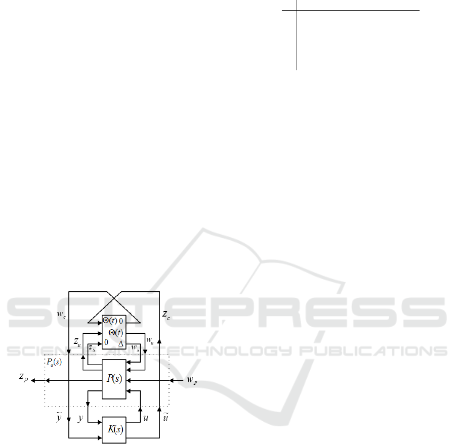
5 SYNTHESIS OF ROBUST LPV

CONTROLLERS WITH LFT

SYSTEM DESCRIPTION

In the following, a robust LPV control with LFT sys-

tem description is developed for a perturbed time–

varying system where the control structure is shown

in Fig.6. The robust control objective is to guaran-

tee some closed loop performance γ > 0 for the L

–

gain of w

→ z

against the time varying measured

Θ(t) and uncertain (not measured) parameters ∆. The

robust LPV control synthesis for LPV systems (both

described with LFT interconnection) should guaran-

tee that the resulting closed loop system is internally

stable for all time varying and uncertain parameters.

Also, the induced L

–norm of the closed loop system

satisﬁes:





∆ 0

0 Θ(t)



(K,Θ(t))





∞

< γ

(21)

where F

and F

are the upper and lower closed loop

system. To solve the above robust LPV synthesis

Figure 6: The robust LPV control structure, LPV system

(s) with the time varying parameters Θ(t) and uncertainty

block ∆

∆

∆.

problem, the uncertainties of the time varying param-

eter vector Θ(t) of both LPV system and controller

are gathered into a single uncertainty block with the

uncertainty ∆ as shown in Fig.6. Here the uncertainty

∆ satisﬁes ∆(iw) ∈ ∆

∆

∆, where ∆

∆

∆ is deﬁned as:

∆

∆ = {∆ = diag[δ

,...,δ

,∆

,...,∆

] : δ

∈ C,

∆

∈ C

×m

∥

∆

∥

< 1} (22)

We introduce the new LTI state–space description

of the system P

(s):







˙x

∆

˜y













A B

0 B

∆

0 D

u∆

0 0 0 0 0 0 I

∆

∆u

0 D

∆∆

∆p

∆1

0 D

p∆

0 D

1∆

0 0 I 0 0 0 0













∆

˜u







(23)

and the LTI controller with a form of :

˙x

= A

+ B



˜y





˜u



= C

+ D



˜y



(24)

so the closed loop system that maps exogenous in-

put w

to controlled output z

can be expressed as:

(s),K(s)), ∆

) (25)

where

∆





∆ 0 0

0 Θ(t) 0

0 0 Θ(t)





, ∆ ∈ C , Θ(t) ∈ R

(26)

The compatible scaling matrix to the block diagonal

uncertainty matrix of (26) is:





∆

0 0

0 D





(27)

where the scaling structure is given as:

∆

∆ = D

∆

∆, ∀∆





Θ(t) 0

0 Θ(t)





Θ(t) 0

0 Θ(t)







, ∀Θ(t)

(28)

The corresponding robust performance problem

can be solved by ﬁnding a robust LTI control in form

of (24) for the nominal LTI system P

(s) of (23)

against the norm bounded structured uncertainties ∆

A sufﬁcient condition for robust performance is pro-

vided by the small gain theorem. This statement is

equivalent to: Given γ > 0, an uncertainty structure

∆

, ﬁnd a scaling matrix D

and an LTI controller

K(s) such that the closed loop system is internally sta-

ble and



1/2

(s),K(s))D

−1/2



∞

< γ (29)

Thus the original LPV control problem is replaced by

a robust control problem admitting some degree of

conservatism.

ICINCO 2022 - 19th International Conference on Informatics in Control, Automation and Robotics

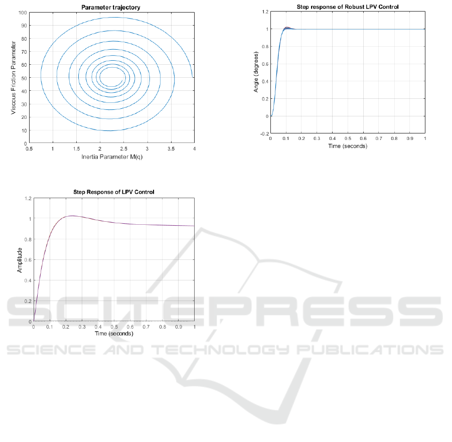
Figure 7: Parameter trajectory.

Figure 8: Step response of the LPV closed loop system.

5.1 Simulation Results of LPV and

Robust LPV Applications

The two parameter M(q) and F( ˙q) are frozen to some

values in the parameter box speciﬁed in (17). The

LPV close loop system is simulated for frozen pa-

rameters 10%, 30%, 60% and 90% of their nominal

values and along the following spiral parameter tra-

jectory shown in Fig.7.

M(q) = 2.25 + 1.7e

−4t

cos(100t) (30)

V (q) = 50 + 49e

−4t

sin(100t)

The step response using LPV control (11) in the pres-

ence of real and dynamic uncertainties is shown in

Fig.8. The step performance is degraded due to the

slow response and high steady state error. The step

response using the robust LPV control (24) shown in

Fig.9 indicates that the performance requirements are

satisﬁed in terms of the steady state and speed of re-

sponse in the presence of same uncertainties.

Figure 9: Step response of the LPV closed loop system with

the presence of uncertainty ∆

∆

∆.

6 CONCLUSIONS

In our research, we developed an LPV control for a

reconﬁgurable manipulator with features such as vari-

able twist angles, length links and hybrid (transna-

tional/rotational) joints. The kinematic design param-

eters, i.e., the D-H parameters, are variable and can

generate any required conﬁguration to facilitate a spe-

ciﬁc application. The dynamic parameters such as in-

ertia, torque and gravity of a reconﬁgurable robot are

dependent on the robot conﬁguration and modeled as

time-varying and can be measured online. An LPV

controller is developed that adapts itself with varying

operating conditions. A robust LPV controllers were

developed using LFT control structure for a perturbed

time-varying system. The closed loop responses us-

ing robust LFT control was proved to satisfy the sta-

bility and tracking performance requirements. This

research is intended to serve as a foundation for fu-

ture studies in reconﬁgurable control systems.

REFERENCES

A. Djuric, R. Al Saidi, W. E. (2010). Global kinematic

model generation of n-dof reconﬁgurable machinery

structure. In Proc. IEEE International Conference on

Automation Science and Engineering.

Apkarian, P. and Adams, R. J. (1997). Advanced gain-

scheduling techniques for uncertain systems. In IEEE

Trans. on Control System Technology, Vol. 6, No. 1,

pp. 21-32.

Kemin Zhou, J. C. Doyle, K. G. (1996). Robust and optimal

control. Printice hall.

P. Gahinet, P. A. (1994). Self-scheduled H

∞

control of linear

parameter varying systems. In Proc. Amer. Control.

Conference. pp. 856-860.

Packard (1994). Gain scheduling via linear fractional trans-

Robust Gain-scheduling LPV Control for a Reconﬁgurable Robot

formations. In Systems and Control Letters, Vol. 22,

pp. 79-92.

Seyed Mahdi Hashemi, Hossam Seddik Abbas, H. W.

(2009). Lpv modelling and control of a 2-dof robotic

manipulator using pca-based parameter set mapping.

In Decision and Control 2009 held jointly with the

2009 28th Chinese Control Conference. Proceedings

of the 48th IEEE Conference on, pp. 7418-7423.

Y.Sun, F.Xu, X. W. and Liang, B. (2018). Lpv model-

based gainscheduled control of a space manipulator.

In the 57th IEEE Conference on Decision and Control

(CDC), FL, USA, December pp. 5114-5120.

Zhongwei Yu, Huitang Chen, P.-Y. W. (2003). Polytopic

gain scheduled H

∞

control for robotic manipulators.

In Robotica volume 21, pp. 495-504.

ICINCO 2022 - 19th International Conference on Informatics in Control, Automation and Robotics