Space-filling Optimization of Excitation Signals for Nonlinear System
Identification
Volker Smits
1 a
and Oliver Nelles
2 b
1
DEUTZ AG, Ottostr. 1, Cologne, Germany
2
Institute of Mechanics and Control - Mechatronics, University of Siegen, Paul-Bonatz-Str. 9-11, Siegen, Germany
Keywords:
Design of Experiment, Genetic Algorithm, Space-filling, System Identification of Multi-variate Nonlinear
Dynamic Systems, Optimal Excitation Signals, APRBS, GOATS, iGOATS.
Abstract:
The focus of this paper is on space-filling optimization of excitation signals for nonlinear dynamic multi-
variate systems. Therefore, the study proposes an extension of the Genetic Optimized Time Amplitude Signal
(GOATS) to multi-variate nonlinear dynamic systems, an incremental version of GOATS (iGOATS), a new
space-filling loss function based on Monte Carlo Uniform Distribution Sampling Approximation (MCUDSA),
and a compression algorithm to significantly speed up optimizations of space-filling loss functions. The results
show that the GOATS and iGOATS significantly outperform the state-of-the-art excitation signals Amplitude
Pseudo Random Binary Signal (APRBS), Optimized Nonlinear Input Signal (OMNIPUS), and Multi-Sine in
the achievable model performances. This is demonstrated on a two-dimensional artificially created nonlinear
dynamic system. Beside the good expectable model quality, the GOATS and iGOATS are suitable for the
usage for stiff systems, supplementing existing data, and easy incorporation of constraints.
1 INTRODUCTION
“A model is worth a thousand datasets” (Rackauckas
et al., 2021). This adage becomes even more obvious
for a special kind of model – the data-based model.
As the name suggests, these models are based on data.
Therefore, they can only represent the information
they can extract from the data used for model train-
ing (Heinz and Nelles, 2017; Heinz et al., 2017; Ti-
etze, 2015). The field of Design of Experiment (DoE)
is well-known for creating experiments to maximize
the amount of information in the data of those experi-
ments. Following the adage “A model is worth a thou-
sand datasets” (Rackauckas et al., 2021), the adage “A
DoE is worth a thousand datasets” also seems appro-
priate.
On the one hand, DoEs can be distinguished by
the purpose of the model whether it shall describe the
transient behavior besides the stationary behavior (dy-
namic DoE) or whether it only shall describe the sta-
tionary behavior (static DoE). On the other hand, a
distinction can be made whether the design is created
offline (passive) DoE or online (active) DoE (Heinz
a
https://orcid.org/0000-0001-8004-7957
b
https://orcid.org/0000-0002-9471-8106
and Nelles, 2017). Popular offline dynamic DoEs
are the step-based excitation signals such as the Opti-
mized Nonlinear Input Signal (OMNIPUS), the Am-
plitude Random Binary Signal (APRBS) (and its vari-
ations), and the sinusoidal-based excitation signals
Chirp and Multi-Sine (Heinz and Nelles, 2017; Heinz
et al., 2017; Hoagg et al., 2006; Nelles, 2013; Tietze,
2015).
One recent study has shown that the global op-
timization approach of a step-based excitation sig-
nal via a genetic algorithm (GA) - Genetic Opti-
mized Amplitude Time Signal (GOATS) - has out-
performed the OMNIPUS, APRBS, Chirp, and Multi-
Sine for three artificially created single-input-single-
output (SISO) nonlinear dynamic systems (Smits and
Nelles, 2021). The objective of the global optimiza-
tion of the GOATS has been a good space-filling cov-
erage of the space X spanned by the system’s inputs
u = [u
1
,u
2
,...,u
p
]
T
and outputs y = [y
1
,y
2
,...,y
o
]
T
.
However, the findings of the study are limited to SISO
systems (Smits and Nelles, 2021).
The present paper aims to add to the current litera-
ture by extending these findings to multi-variate non-
linear dynamic systems. In this study, we also aim to
develop a novel step-based signal which combines the
advantages of the OMNIPUS and GOATS in order to
Smits, V. and Nelles, O.
Space-filling Optimization of Excitation Signals for Nonlinear System Identification.
DOI: 10.5220/0011338700003271
In Proceedings of the 19th International Conference on Informatics in Control, Automation and Robotics (ICINCO 2022), pages 255-262
ISBN: 978-989-758-585-2; ISSN: 2184-2809
Copyright
c
 2022 by SCITEPRESS – Science and Technology Publications, Lda. All rights reserved
255

weaken one major disadvantage of the OMNIPUS.
The OMNIPUS’s major advantage is its incre-
mental design so that the subsequences of the sig-
nal are space-filling. The GOATS’s main advantage
is its high degree of freedom due to the utilization
of a global approach. Unfortunately, with the advan-
tage of the OMNIPUS also comes the disadvantage
of a lack in the degree of freedom. That is, in ev-
ery iteration, OMNIPUS optimizes only one ampli-
tude of one input. To overcome this limitation and
to weaken the resulting disadvantage of previous sub-
optimal optimized sequences, an incremental version
of the GOATS (iGOATS) is developed by considering
a bigger and more complex subsequence inside one
iteration. The iGOATS optimizes all inputs simul-
taneously and the number of subsequent steps con-
sidered in one iteration can be selected by the user.
In addition, five loss functions are examined for the
optimization of the GOATS and iGOATS including
a novel space-filling loss function based on Monte
Carlo Uniform Distribution Sampling Approximation
(MCUDSA). Furthermore, a compression approach is
developed to speed up the space-filling optimization.
For better visualization, the investigation is shown
on an artificial nonlinear first-order dynamic multi-
input-single- output (MISO) system with two inputs
(p = 2, o = 1).
The present paper is structured as follows. First,
the methods are introduced and explained. The
method section starts with the signal types developed
by the authors – GOATS and iGOATS. After that,
the loss functions, optimization problems, and GAs
which are used for optimization of the GOATS and
iGOATS are introduced. Following that, the compres-
sion algorithm for the speed up of the optimization
is illustrated. The last section of the method section
deals with the modeling approach which is used for
model training according to the different excitation
signals.
The experiment section describes the investigated
artificial process and the concrete design of the exci-
tation signals and the test signal. After that, the dif-
ferent excitation signals are analyzed in their space-
filling property and their achieved model quality. At
the end, a conclusion and an outlook are given.
2 METHOD
2.1 Signal Types
GOATS. The GOATS is a global optimized ex-
citation signal where the occurrence and the dura-
tion of predefined amplitude levels e.g., via a static
GOATS
amplitude
modulation
1
0
0.0 1.00.2 0.4 0.6 0.8
6 21 4 3 5
2 23 4 1 5
GA
amplitudes
1 62 3 4 5
Figure 1: Example of a GOATS.
DoE method like an optimal Latin Hypercube (LHC)
are optimized (Bates et al., 2004; Smits and Nelles,
2021). The design of the GOATS is illustrated in
Fig. 1. The optimization parameters of the GOATS
are the permutation of the predefined amplitude lev-
els θ
p
and the duration of each level θ
d
(Smits and
Nelles, 2021).
iGOATS. The iGOATS is an incremental global op-
timized excitation signal. It optimizes all inputs si-
multaneously and the number of subsequent steps
can be defined by the user. The following pseudo-
code illustrates the procedure. It starts with an ini-
Algorithm 1: iGOATS algorithm.
Step 1: Initialize sequence
while N < N
des
do
Step 2: Start GA with current sequence
Step 3: Append sequence with a subsequent
steps of h optimized subsequent steps via
the GA
end while
tial sequence e.g., with the upper limits of the in-
puts or already existing data. In every loop, a sub-
sequence for every input dimension is optimized si-
multaneously and appended to the existing sequence.
The number of subsequent steps h in a single iter-
ation of the iGOATS algorithm can be chosen by
the user. Furthermore, the user can specify whether
all h subsequent steps should be appended or only
a steps should be appended. Theoretically, the last
step does not benefit from the planning feature for
the next step if all subsequent steps a = h are at-
tached. Conversely, the last attached step is not neg-
atively affected by the simultaneous planning of the
next step and the planning by its predecessor. The
planning feature is given when at least two subse-
quent steps h = 2 are considered. Note that, the
computational demand significantly rises when only
a = h − 1 steps are appended, because more itera-
tions are necessary to reach the desired signal length
N
des
. The amplitude levels Θ
a
= [θ
a,1
,...,θ
a,p
] and
durations for the levels Θ
d
= [θ
d,1
,...,θ
d,p
] of the h
subsequent steps are the optimization parameters of
the iGOATS, where θ
a,v
= [θ
a,v
(1),...,θ
a,v
(h)]
T
and
θ
d,v
= [θ
d,v
(1),...,θ
d,v
(h)]
T
.
ICINCO 2022 - 19th International Conference on Informatics in Control, Automation and Robotics
256

0
1
0
1
0
1
u
1
u
2
ˆy
OMNIPUS
0
1
0
1
0
1
u
1
u
2
iGOATS(h=1, a=1)
0
1
0
1
0
1
u
1
u
2
ˆy
iGOATS(h=2, a=2)
0
1
0
1
0
1
u
1
u
2
iGOATS(h=2, a=1)
Figure 2: Comparison of OMNIPUS and iGOATS for the
first five steps. The green line denotes the initial sequence.
Note that, the resulting independent sequences
u
1
,...,u
p
have to be concatenated for model evalu-
ation and the shortest sequence length will define the
signal duration.
A good example for the disadvantages of the
OMNIPUS and the planning feature of the iGOATS
can be extracted by comparing the diagrams of
Fig. 2. Figure 2 shows the point distribution of the
two-dimensional system described by the Eq. (12)
- Eq. (17) for the excitation via OMNIPUS and
iGOATS. In comparison to the iGOATS, the OMNI-
PUS cannot reach the input combination (u
1
= 0, u
2
=
1) in the first five steps since it does not simultane-
ously optimize both inputs. The OMNIPUS needs
several steps to drive the systems towards to the upper
left corner.
The lower diagrams show the iGOATS with two
subsequent steps h. Step four and five of the
iGOATS (h = 2, a = 2) and step three and four of
the iGOATS (h = 2, a = 1) steer the model output ˆy
respectively the system output y towards one just to
drive it with step five respectively step four towards
zero. This results in a transient response more close
to the upper left corner (u
1
= 0, u
2
= 1, ˆy ≈1) which
would not be reached without the planning feature
(see iGOATS (h = 1, a = 1)). As illustrated in Fig. 2
the space-filling property of the iGOATS (h = 2, a =
2) and iGOATS (h = 2, a = 1) does not differ much.
2.2 Loss Functions and Optimization
Problems
Loss Functions. The optimization objectives for
the genetic optimization are the cross correla-
tion between the input sequences (see Eq. 5)
and the space-filling property of the space X =
[u
1
,...,u
p
,y
1
,...,y
o
] spanned by the system’s inputs
u
v
= [u
v
(1),...,u
v
(N)]
T
, where v = 1,..., p and out-
puts y
m
= [y
m
(1),...,y
m
(N)]
T
, where m = 1, . . . , o.
Therefore, X ∈ R
N×n
where N defines the number
of samples respectively the signal duration and n the
number of inputs and outputs. Examples of space-
filling optimized sequences are illustrated in Fig. 2
and Fig. 4. Note, that for the optimization of the
space-filling criteria a proxy model (in this study a
linear proxy model) ˆy(u) is needed to roughly approx-
imate the system’s outputs (
˜
X = [u
1
,...u
p
, ˆy
1
..., ˆy
o
],
˜
X ∈ R
N×n
).
The space-filling loss functions can be further sub-
divided into designs inspired by maximin design (AE,
Eq. (1) and MMNS, Eq. (2)) and designs which try
to approximate a uniform distribution (MCUDSA,
Eq. (2) and FA, Eq. (4)). The loss functions inspired
by maximin design penalize too close points. The
MCUDSA and FA losses try to minimize deviation
to a uniform distribution. Therefore, they make use
of support points S which approximate space-filling
coverage in the unit cube (S ∈ R
M×n
). Thereby, M
defines the number of support points. In this study,
S which is used during the optimization is created by
M = 1000 points via the static DoE method optimal
LHC (Bates et al., 2004). The following list summa-
rizes the loss function equations. Note that, the i-th
row of a matrix e.g.,
˜
X is defined as ˜x
T
i
.
• Audze Eglais (AE) (Audze and Eglais, 1977)
L
AE
= N
2
N(N −1)
N
∑
i=1
N
∑
k=i+1
(
k
˜x
i
−˜x
k
k
2
)
−2
(1)
• Maximum Nearest Neighbor Sequence (MNNS)
(Heinz et al., 2017)
L
MNNS
= −
1
L
N+L
∑
k=N+1
min(
k
(˜x
i
−˜x
k
k
2
) (2)
+ #u
v,l
v
d
max
,∀i ∈ {1,...,N}
• Monte Carlo Uniform Distribution Sampling Ap-
proximation (MCUDSA)
L
MCUDSA
=
N
M
N
∑
i=1
min(
k
˜x
i
−s
k
k
2
), (3)
∀k ∈{1,. . .,M}
• Fast and Simple Dataset Optimization (FA) (Peter
and Nelles, 2019; Smits and Nelles, 2021)
L
FA
= N
N
∑
i=1
|1 − ˆq(˜x
i
)|, (4)
ˆq(˜x
i
) =
1
M
N
∑
i=1
e
−
1
2
[s
k
−˜x
i
]
T
Σ
−1
[s
k
−˜x
i
]
p
(2π)|Σ|
∀k ∈{1,. . .,M},Σ = diag(σ
2
1
,σ
2
2
,...,σ
2
n
)
Space-filling Optimization of Excitation Signals for Nonlinear System Identification
257

• Cross correlation of the input sequences (XCor)
L
XCor
=
2
p(p −1)
p
∑
v=1
p
∑
j=i+1
(u
v
∗u
j
)[l] (5)
(u
v
∗u
j
)[l] =
N
∑
i=1
u
v
(i)u
j
(i + l)
where time lag l = 0
The term +#u
v,l
v
d
max
of Eq. (2) denotes a LHC-
based penalization term which can be used to ensure a
non-collapsing design. Thereby, #u
v,l
v
represents the
counter of already chosen amplitude levels for each
input dimension and d
max
=
√
n a factor to weigh the
counter (Heinz et al., 2017)
1
. L in (2) defines the over-
all length of subsequent steps.
The original calculation of the FA is slightly
adapted by the use of supporting points instead of the
data set itself to decouple the pdf estimation of the
data set. The ˆq of the FA loss function L
FA
can be
interpreted as a n-dimensional pdf estimation where
the kernels are placed on the supporting points S.
The standard deviations σ of the covariance matrix
Σ of Eq. (4) are calculated by the Silverman‘s rule-of-
thumb (Silverman, 1986).
Note, that all loss functions are constructed as
minimization problems and the multiplication with N
in the Eq. (1), Eq. (3), and Eq. (4) is performed to pro-
duce a trade-off between the signal duration and the
space-filling coverage.
Optimization Problems. While the iGOATS only
uses the MNNS loss function for optimization, the
GOATS is examined for the three space-filling loss
functions (AE, MCUDSA, FA) in a single objective
optimization and in a multi objective optimization ac-
cording to the AE and XCor loss functions. Note
that, changes in θ
p
,θ
d
, Θ
a
, and Θ
d
result in differ-
ent system inputs u
1
,...,u
p
. Consequently, it also re-
sults in different proxy model outputs ˆy
1
,..., ˆy
o
and
in changes in the matrix
˜
X.
single-GOATS : min
θ
p
,θ
d
( f (
˜
X(θ
p
,θ
d
))) (6)
multi-GOATS : min
θ
p
,θ
d
( f
AE
(
˜
X(θ
p
,θ
d
)), (7)
f
XCor
(u
1
(θ
p
,θ
d
),...,u
p
(θ
p
,θ
d
)))
single-iGOATS : min
Θ
a
,Θ
d
( f
MNNS
(
˜
X(Θ
a
,Θ
d
))) (8)
1
(Heinz et al., 2017) addresses the topic more compre-
hensive, l
v
denotes the level index
2.3 Genetic Algorithm
GAs are meta-heuristic global optimizers which are
capable of simultaneously optimizing several param-
eter types respectively encodings like permutations,
real-valued arrays, integer arrays, and binary rep-
resentations of real and integer values (which in-
clude the parameter types of the signals GOATS and
iGOATS) without needing a gradient which makes
them suitable to optimize all of the proposed loss
functions. For the single objective optimization via
the GA the diversity-guided genetic algorithm is used
(Ursem, 2002). The diversity div of the population is
calculated by the mean of the standard deviation of
each parameter type
2
of all individuals of the popula-
tion.
div =
1
K
K
∑
k=1
σ
k
(9)
The diversity guided GA differs from the procedure of
a simple GA through its separation of the genetic op-
erators crossover and mutation in one generation con-
trolled by a diversity mechanism (high diversity →
crossover, low diversity → mutation) (Ursem, 2002).
As the selection scheme for single objective op-
timization the popular Tournament Selection is ap-
plied (Goldberg and Deb, 1991; Razali and Geraghty,
2011). In contrast to the diversity-guided GA of sin-
gle objective optimization, the multi objective opti-
mization problems are optimized via the Non Domi-
nated Sorting Algorithm II (NSGA II) without diver-
sity guiding (Deb et al., 2000). Instead, the probabil-
ity for the crossover and mutation is calculated adap-
tively inspired by the work of Lin (Lin et al., 2003).
The crossover and mutation operators for the
GOATS are chosen as in (Smits and Nelles, 2021).
The real and natural number parameter types of
the iGOATS are represented in a binary encoding.
For this binary representation, the well-known single
point crossover and flip mutation is used (Sivanandam
and Deepa, 2008). The selection of genetic opera-
tors in this study is done experimental on the present
problem and omitted in this contribution to conserve
space.
2.4 Compression
The following compression algorithm is designed to
speed up the evaluation of the space-filling loss func-
tions. The speed up is achieved through considering
not all N data points for the loss functions but only
the most relevant in a space-filling sense. The general
2
e.g., for GOATS: θ
p
and θ
d
, K :=number of parameter
types
ICINCO 2022 - 19th International Conference on Informatics in Control, Automation and Robotics
258

idea of the compression algorithm is first to divide the
time series of the system’s output in the time domain
by critical points and then to select the data points be-
tween the critical points uniformly in y-direction. The
following pseudo code gives an overview of the gen-
eral procedure. It is to note, that the critical points can
Algorithm 2: Compression algorithm.
1. Step: Normalize system response
2. Step: Identify critical points c
3. Step: Calculate distances ∆ in
y-direction between critical points c
4. Step: Select n
i
= ∆
i
· α space-filling
points between c
i
and c
i+1
for i=1:number of critical points-1 do
4.1 Step: Create linear slope between c
i
and c
i+1
with n
i
points
4.2 Step: Select nearest neighbor
(smallest ∆y) for each point of the slope
in y between c
i
and c
i+1
end for
5. Step: Concatenate critical and
space-filling points
be identified in several ways. For aperiodic system re-
sponses – excited via a step-based excitation signal –
only the points where the steps occur are sufficient.
If the system response is not aperiodic or non-step-
based excitation signals are used, the critical points
can be identified by curve analysis (e.g., finding sign
changes in the gradient ∆y(t)/∆t, finding maximum
curvatures ∆
2
y(t)/∆
2
t) or by an consideration of de-
viations of the integrals between the true
R
y(t) dt and
an approximated version
R
˜y(t) dt (e.g., by a linear ex-
trapolation of the last two critical points). The number
of points n
i
which are selected between two critical
points is calculated by the product of ∆
i
and a user-
defined factor α.
3
Fig. 3 shows an illustration of the compression al-
gorithm for a subsection of the system response of the
linear proxy model excited by OMNIPUS. The pa-
rameters for the compression algorithm in this study
has been chosen to α = 10 and only the step position
as critical points has been used. Beside the selected
points in Fig. 3, the critical points are selected as well
as mentioned in Algorithm 2.
Table 1 summarizes the comparison of the evalua-
tion speed for different loss functions and for several
number of points. The experiments are performed on
the linear proxy model of the present process. Ta-
ble 1 shows that a reduction of the evaluation speed
can be achieved by compression. The reduction is sig-
nificantly and lies in the range from 3.8 to 15 times.
3
∆ denotes the vector of differences in y-direction be-
tween each critical point
0 10 20 30 40 50
0
0.25
0.5
0.75
1
∆y
∆
i
samples
system output y
Figure 3: Compression example, red: critical points, or-
ange: selected points, green: slope points.
Table 1: Comparison of the compression effect for the
space-filling loss function. Evaluation time of compressed
data in ms - Compared on an Intel Core i7-8750 @
2.20GHz with the Julia Programming Language (Bezanson
et al., 2017).
loss number of points speed up
functions 500 1000 2000 factor
AE 0.02 0.07 0.28 15
MCUDSA 9.13 21.7 52.6 5.5
MNNS 0.49 0.91 1.77 3.8
FA 28.2 87.1 148 4.5
compression
0.10 0.20 0.38
algorithm
For an optimization in a global manner, like for the
GOATS, the evaluation speed of algorithm itself is
important. It reduces the accelerations to the range
from 3 to 6 times.
Another interesting question is: How does the
compression affects the space-filling optimization?
Exemplary, the deterministic optimization of the OM-
NIPUS is consulted for this analysis. Fig. 4 shows the
effect of the compression on the space-filling prop-
erty of the OMNIPUS. The point distribution is nearly
identical because no important data points are omit-
ted by the compression. Hence, the compression has
no negative effect on the optimization. Therefore, it
is carried out for all optimization of all signal types
where a space-filling loss function is used.
2.5 Modeling Approach
Beside the discussed loss functions, one could won-
der how to quantify the quality of an excitation sig-
0
0.5
1
0
0.5
1
input u
1
input u
2
0
0.5
1
0
0.5
1
input u
1
model output ˆy
0
0.5
1
0
0.5
1
input u
2
model output ˆy
Figure 4: Effect of compression during optimization of
OMNIPUS.
Space-filling Optimization of Excitation Signals for Nonlinear System Identification
259

nal. One straightforward and reasonable approach is
to compare the model qualities which can be achieved
by the excitation signals. This approach of rating
the excitation signals is too computational expensive
to use it directly in an optimization, but for rating
the results it is appropriate. Therefore, a determin-
istic model training is preferable, because a stochas-
ticity during training impedes the analysis (Smits and
Nelles, 2021).
A model architecture which can be optimized via
a deterministic training algorithm – Hierarchical Lo-
cal Model Tree (HILOMOT) – is the architecture of
Local Model Networks. It achieves good model qual-
ities and does not need much hyperparameter tuning
(Nelles, 2013, 2006). HILOMOT divides the space
incrementally in an axis-oblique manner and con-
structs local models in the subspaces. A sum of the
outputs of the local models ˆy
i
(x) weighted by the val-
idation functions Φ
i
(z) results in the overall model
output ˆy. Thereby, x and z are defined by the user
as subsets of all inputs u (Nelles, 2006):
ˆy(x,z) =
M
∑
i=1
ˆy
i
(x) ·Φ
i
(z) , where
M
∑
i=1
Φ
i
(z) = 1. (10)
3 EXPERIMENT
3.1 Process
The experiment examines a two-dimensional nonlin-
ear artificially created dynamic system. The investi-
gated process is a superposition of a first-order Ham-
merstein process with an arctangent function as sta-
tionary nonlinearity and a first-order Wiener process
with a quadratic function as stationary nonlinearity.
Therefore, it yields strong enough nonlinearities and
dynamic aspects for a proper investigation of the ex-
citation signals with multiple inputs. The dominant
time constants of the process for each input are iden-
tified by step responses (T
1
= 0.5 s and T
2
= 1.6 s).
Derived from the system response of linear first-order
time-invariant system, the length of one subsequence
is limited to the following interval.
T
i
/T
0
< L
i
< 3pT
i
/T
0
(11)
The following equations define the process.
y(k) = 0.5y
1
(k) + 0.5y
2
(k) (12)
y
1
(k) = 0.2 f
1
(u
1
(k −1)) + 0.8y(k −1) (13)
y
2
(k) = f
2
(v(k)) (14)
v(k) = 0.1u
2
(k −1) + 0.9v(k −1) (15)
f
1
(x) =
atan(8x −4) + atan(4)
2atan(4)
(16)
f
2
(x) = x
2
(17)
The process will be excited in the amplitude range
of (0.0, 1.0) for both inputs and a sample period of
T
0
= 0.1s is considered.
3.2 Training Signals and Test Signals
Training Signals. All training signals (APRBS,
Multi-Sine, OMNIPUS, GOATS, and iGOATS) are
investigated for different durations and compared on
their space-filling property and their achievable model
quality on the test data which is described later.
The OMNIPUS and iGOATS are incremental so
that every subset can be used. For both signals, the
LHC-based penalization term is used for a better com-
parison to the APRBS and GOATS. The hyperparam-
eter settings for the OMNIPUS are derived from the
suggestions of Heinz and Nelles (Heinz et al., 2017).
The number of subsequent steps h of the iGOATS
considered for optimization and appending in a sin-
gle iteration has been chosen to two in order to en-
able the planning capability. The appending of only
a = h −1 subsequent steps has been analyzed but it
has not shown an advantage for this investigation.
The durations of the GOATS and APRBS are
mainly influenced by number of amplitude levels
which are used. Therefore, three numbers of ampli-
tude levels 25, 50, and 100 are investigated to achieve
different durations.
The APRBSs share the same amplitude levels as
the GOATSs while the permutations of the levels are
random and the dwell time is chosen to 1 s. Further-
more, one APRBS with an average model quality on
the test data for each number of amplitude levels has
been selected of a set of 100 APRBSs for comparison.
The Multi-Sines are created for different dura-
tions in the interval t
stop
= 10 s −100 s within a fre-
quency interval of 0.01 Hz −1 Hz and an optimized
Schroeder Phase (Schroeder, 1970). The number of
sine waves considered for each Multi-Sine is calcu-
lated by 0.75t
stop
/s. In addition, the Multi-Sines for
the input u
1
and u
2
are optimized in their cross corre-
lation.
Test Signal. The test signal is a combination of
APRBS, Ramp (Tietze, 2015), Chirp, and Multi-Sine
with equal durations of 100 s each to cover differ-
ent aspects of the process. The chosen dwell time
for the APRBS and Ramp is 1s. The Chirp and
Multi-Sine are designed in the frequency range of
0.01Hz −1 Hz.
ICINCO 2022 - 19th International Conference on Informatics in Control, Automation and Robotics
260

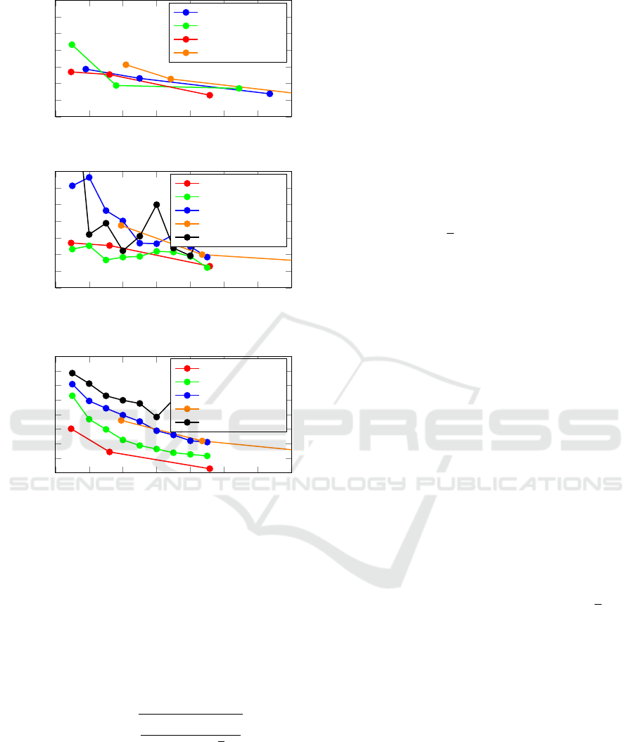
10 30 50 70 90 110 130 150
0.18
0.2
0.22
0.24
0.26
0.28
0.3
0.32
(191, 0.2)
NRMSE
GOATS
AE
GOATS
FA
GOATS
MCUDSA
GOATS
AE+XCor
(a) Different GOATS compared by NRMSE
10 30 50 70 90 110 130 150
0.18
0.2
0.22
0.24
0.26
0.28
0.3
0.32
(195, 0.2)
NRMSE
GOATS
MCUDSA
iGOATS
OMNIPUS
APRBS
MultiSine
(b) Best signals compared to state-of-the-art signals by
NRMSE
10 30 50 70 90 110 130 150
0.1
0.12
0.14
0.16
0.18
0.2
0.22
0.24
0.26
(195, 0.121)
time (s)
MCUDSA
GOATS
MCUDSA
iGOATS
OMNIPUS
APRBS
Multi-Sine
(c) Best signals compared to state-of-the-art signals by
MCUDSA
Figure 5: Comparison of excitation signals for different du-
rations.
4 ANALYSIS OF THE TRAINING
SIGNALS
The model performance is measured by the Normal-
ized Root Mean Squared Error (NRMSE)
NRMSE =
s
∑
N
i=1
(y(i) − ˆy(i))
2
∑
N
j=1
(y( j) −y)
2
(18)
of the test data. Fig. 5 shows the model performances
and the space-filling property of the investigated train-
ing signals.
First, in Fig. 5a the different optimizations of the
GOATS are compared according to the NRMSE on
the test data. The GOATS
MCUDSA
outperforms the
GOATS
AE
, GOATS
FA
, and GOATS
AE+XCor
for short
signal durations. Additionally, the optimizations ac-
cording to MCUDSA result in shorter excitation sig-
nals with a comparable or superior performance com-
pared on the number of amplitude levels (25, 50, 100).
The multi objective optimization according to AE and
XCor does not have a better influence on the model
performance compared to the single objective accord-
ing to AE. One explanation might be, that the separate
influences of u
1
and u
2
on y can be extracted suffi-
ciently from the data, even when the cross correlation
of u
1
and u
2
is not optimized. Note that, the “best”
solution for the multi objective optimization has been
taken by normalizing the resulting pareto front of op-
timization and selecting the individual with the fitness
closest to the origin 0.
Consequently, the overall winner GOATS
MCUDSA
is compared according to the NRMSE on the test data
in Fig. 5b to the iGOATS, OMNIPUS, APRBS, and
the Multi-Sine. Fig. 5b shows, that the GOATS and
iGOATS significantly surpass the Multi-Sine in the
model performance on the test data for short signal
durations.
Higher NRMSE values than 0.32 are omitted in
Fig. 5 for better visibility of the performance of exci-
tation signals. The iGOATS and GOATS
MCUDSA
have
comparable model performances and they outperform
the performance of the OMNIPUS e.g., by approxi-
mately 34% for the signal duration of 20s and 20 %
for the signal duration of 50s which is even more sig-
nificant compared to the findings in (Smits and Nelles,
2021). This can be explained by the higher degree of
freedom of the approaches and the higher input di-
mension as in (Smits and Nelles, 2021). Due to the
higher degree of freedom, the iGOATS and GOATS
have a better space-filling property which is depicted
in Fig. 5c. Fig. 5c shows the MCUDSA loss func-
tion values without the factor N for different durations
evaluated on 2
15
= 32768 supporting points S gen-
erated via a Sobol sequence (Bratley and Fox, 1988;
Joe and Kuo, 2003). Furthermore, the iGOATS and
GOATS exceed the average NRMSE of an APRBS
illustrated in Fig 5b, e.g., by 15 % for the signal dura-
tion of 50s which is similar to the findings in (Smits
and Nelles, 2021). At this point, it should be noted
that APRBSs also often provide worse model per-
formances than the average performance, especially
for short signal durations. In contrast, the GOATS,
iGOATS, and OMNIPUS overcome this disadvantage
due to an ensured good coverage of the space. There-
fore, they deliver a reliable expectable model perfor-
mance.
Space-filling Optimization of Excitation Signals for Nonlinear System Identification
261

5 CONCLUSION
The present study has aimed to extend the GOATS to
multi-variate nonlinear dynamic systems, to develop a
new signal type iGOATS, to create a new space-filling
loss function MCUDSA, and to produce a compres-
sion algorithm to significantly speed up optimizations
of space-filling loss functions.
The GOATS has been successfully extended to
multi-variate nonlinear dynamic systems with a supe-
rior expectable model quality and space-filling prop-
erty.
Furthermore, a new signal type – iGOATS –
has been developed. The iGOATS combines the
good expectable model qualities of the GOATS with
the incremental feature of the OMNIPUS. Conse-
quently, the GOATS and iGOATS surpass the OM-
NIPUS, APRBS, and Multi-Sine significantly espe-
cially for short signal durations on the artificially two-
dimensional nonlinear dynamic process.
The new space-filling loss function MCUDSA for
the optimization of the GOATS slightly outperforms
the AE and FA loss functions in this investigation.
However, for greater and more complex systems the
AE might be interesting as well due to the faster eval-
uation speed and optimization.
The approach to accelerate the optimization speed
of space-filling loss functions for dynamic DoEs via
compressing the data shows that the evaluation can
be sped up between 3 −6 times according to the used
loss function including the computational effort of the
compression algorithm itself.
In future research, the GOATS and iGOATS have
to be examined for higher dimensional, higher order
and real world dynamic nonlinear systems.
REFERENCES
Audze, P. and Eglais, V. (1977). New approach for plan-
ning out of experiments. Problems of Dynamics and
Strengths, 35:104–107.
Bates, S. J., Sienz, J., and Toropov, V. V. (2004). Formula-
tion of the optimal latin hypercube design of experiments
using a permutation genetic algorithm. In Collection of
Technical Papers - AIAA/ASME/ASCE/AHS/ASC Struc-
tures, Structural Dynamics and Materials Conference,
volume 45.
Bezanson, J., Edelman, A., Karpinski, S., and Shah, V. B.
(2017). Julia: A fresh approach to numerical computing.
SIAM review, 59(1):65–98.
Bratley, P. and Fox, B. L. (1988). Algorithm 659: Im-
plementing Sobol’s Quasirandom Sequence Generator.
ACM Transactions on Mathematical Software (TOMS),
14(1):88–100.
Deb, K., Agrawal, S., Pratap, A., and Meyarivan, T. (2000).
A fast elitist non-dominated sorting genetic algorithm
for multi-objective optimization: NSGA-II. In Interna-
tional conference on parallel problem solving from na-
ture, pages 849–858.
Goldberg, D. E. and Deb, K. (1991). A Comparative Anal-
ysis of Selection Schemes Used in Genetic Algorithms.
Foundations of genetic algorithms, 1:69–93.
Heinz, T. O. and Nelles, O. (2017). Iterative Excitation Sig-
nal Design for Nonlinear Dynamic Black-Box Models.
Procedia Computer Science, pages 1054–1061.
Heinz, T. O., Schillinger, M., Hartmann, B., and Nelles, O.
(2017). Excitation signal design for nonlinear dynamic
systems with multiple inputs – A data distribution ap-
proach. In R
¨
opke, K. and G
¨
uhmann, C., editors, Inter-
national Calibration Conference - Automotive Data An-
alytics, Methods, DoE, pages 191–208. expertVerlag.
Hoagg, J. B., Lacy, S. L., Babu
ˇ
ska, V., and Bernstein, D. S.
(2006). Sequential multisine excitation signals for sys-
tem identification of large space structures. In Proceed-
ings of the American Control Conference, pages 418–
423.
Joe, S. and Kuo, F. Y. (2003). Remark on Algorithm 659:
Implementing Sobol’s quasirandom sequence generator.
ACM Transactions on Mathematical Software, 29(1):49–
57.
Lin, W. Y., Lee, W. Y., and Hong, T. P. (2003). Adapting
crossover and mutation rates in genetic algorithms. Jour-
nal of Information Science and Engineering, 19:889–
903.
Nelles, O. (2006). Axes-Oblique Partitioning Strategies for
Local Model Networks. In IEEE International Sympo-
sium on Intelligent Control, pages 2378–2383. IEEE.
Nelles, O. (2013). Nonlinear system identification: from
classical approaches to neural networks and fuzzy mod-
els. Springer Science & Business Media.
Peter, T. J. and Nelles, O. (2019). Fast and sim-
ple dataset selection for machine learning. at-
Automatisierungstechnik, 67(10):833–842.
Rackauckas, C., Ma, Y., Martensen, J., Warner, C., Zubov,
K., Supekar, R., Skinner, D., Ramadhan, A., and Edel-
man, A. (2021). Universal differential equations for sci-
entific machine learning.
Razali, N. M. and Geraghty, J. (2011). Genetic algorithm
performance with different selection strategiesin solving
TSP. In Proceedings of the World Congress on Engineer-
ing, volume 2, pages 1–6.
Schroeder, M. (1970). Synthesis of low-peak-factor sig-
nals and binary sequences with low autocorrelation
(corresp.). IEEE Transactions on Information Theory,
16(1):85–89.
Silverman, B. W. (1986). Density estimation for statistics
and data analysis. CRC press, 26.
Sivanandam, S. N. and Deepa, S. N. (2008). Introduction to
genetic algorithms. Berlin: Springer.
Smits, V. and Nelles, O. (2021). Genetic optimization of
excitation signals for nonlinear dynamic system identifi-
cation. In Proceedings of the 18th International Confer-
ence on Informatics in Control, Automation and Robotics
- ICINCO, pages 138–145. INSTICC, SciTePress.
Tietze, N. (2015). Model-based calibration of engine con-
trol units using gaussian process regression. PhD thesis,
Technische Universit
¨
at Darmstadt.
Ursem, R. (2002). Diversity-Guided Evolutionary Algo-
rithms. In Parallel Problem Solving from Nature —
PPSN VII, pages 462–471.
ICINCO 2022 - 19th International Conference on Informatics in Control, Automation and Robotics
262