
Adaptive Fault Detection and Isolation for DC Motor Input and
Sensors
Nikita Kolesnik
a
, Alexey Margun
b
, Artem Kremlev
c
and Andrei Zhivitskii
1d
Control Systems and Robotics Dept., ITMO University Saint Petersburg, Russia
Keywords: Fault Detection, Fault Isolation, DC Motor, Identification, Adaptive System.
Abstract: The paper is devoted to the development of an adaptive approach to the fault detection and isolation of input
and sensor failures of armature-controlled direct current motors. The proposed detection method is based on
the full state Luenberger observer. Isolation scheme uses the directional residual set and relationships between
fault directions and residual vector. Adaptability is provided by dynamic regressor extension and mixing
approach for online estimation of parameters. Proposed scheme allows to isolate following faults:
unaccounted load acting on the rotor, input voltage disturbance, failures of velocity and current sensors.
Simulation results confirm performance of the proposed approach.
1 INTRODUCTION
The development of technologies leads to use of
process automation systems in various fields of
human activity: industrial manufacturing,
autonomous cars and aircrafts, HVAC, etc. These
systems typically have a complex structure that
includes interconnected sensors, actuators and
passive elements. Failures of system parts may cause
sufficient consequences. Therefore, timely fault
detection and isolation is of particular importance,
especially for safety-critical systems. Such function
allows to increase reliability, perform predictive
maintenance, effective reconfiguration and quick
failure elimination. According to Wunnenberg (1990)
faults can be classified as follows: com- ponent fault
(deviation of a plant parameters from its nominal
values); sensor fault (sensor measurement doesn’t
corresponds to real physical value); actuator fault
(deviation of control signals from the desired values).
The most common methods of fault detection are
observer based approaches, parity relations,
parameter identification based algorithms and
machine learning approaches (Chen & Patton, 1999).
Parity relation methods rely on hardware or temporal
redundancy. Hardware duplication is effective and
a
https://orcid.org/0000-0002-8630-4202
b
https://orcid.org/0000-0002-5333-0594
c
https://orcid.org/0000-0002-7024-3126
d
https://orcid.org/0000-0002-0632-778X
does not require system model but demands
additional financial costs for adding sensor and
maintenance (Ray & Luck, 1991). Another drawback
of a sensor duplication is a confines imposed by
technological restrictions. Temporal redundancy
requires accurate plant model, but doesn’t need
additional hardware devices. Both approaches have a
good performance for sensor faults detection in linear
systems and are applicable for DC motors.
Observer based approaches use difference
between estimated and measured state variables
(residual) for fault detection. Isolation problem can be
solved with structured and directional residual sets or
fault detection filters (Patton & Chen, 1997). The
structured set method is based on synthesis of specific
residual generator sensitive for only one or all-but-
one corresponding fault. The main idea of directional
generators set is changing of residual signals in only
one direction that corresponds to the specific fault in
a residual space. Fault direction filters approaches use
special procedures of observer synthesis to make it
sensitive to the specific failures. Mentioned above
methods are effective for actuator and sensor fault
detection and isolation (Chung & Speyer, 1998).
Problem of robustness with respect to the
parametric uncertainties, disturbances, noises and
Kolesnik, N., Margun, A., Kremlev, A. and Zhivitskii, A.
Adaptive Fault Detection and Isolation for DC Motor Input and Sensors.
DOI: 10.5220/0011336700003271
In Proceedings of the 19th International Conference on Informatics in Control, Automation and Robotics (ICINCO 2022), pages 703-710
ISBN: 978-989-758-585-2; ISSN: 2184-2809
Copyright
c
2022 by SCITEPRESS – Science and Technology Publications, Lda. All rights reserved
703

additive nonlinearities can be solved with the use of
unknown input observers (Chen, Patton & Zhang).
However, the synthesis procedure for these
algorithms has solution only for a class of linear
systems with sufficient limitations on plant matrices.
Model of DC motor with measured velocity or current
doesn’t satisfy the necessary conditions
(Wunnenberg, 1990).
Identification approaches use online parameters
estimation algorithms (for example, gradient descent
or least squares). These methods provide detection
and isolation of component faults on the base of
deviation between nominal and estimated parameters
(Isermann, 1997).
Last researches propose to use artificial
intelligence and neural networks to detect and isolate
faults. In (Santos et all, 2018) the fault detection and
classification schemes are proposed. The fault is
detected by a classical Luenberger observer. The
classification is based on a representation which
combines the subctrative clustering algorithm with an
adaptation of particle swarm clustering. DC motor
fault detection, isolation and identification based on a
neural networks approach is presented in (Adouni,
Abid & Sbita, 2016). However, this method requires
a lot of computational power and don’t guarantee
results. Experimental researches of fault detection
and diagnosis methods for DC motor drives are
analyzed in (Isermann, 2006).
This paper is devoted to the actuator and sensor
adaptive fault detection and isolation for armature
controlled direct current motors. Unknown input
observers don’t exist in the cases of sensor and
actuator faults occurring in mechanical and electrical
parts (equations for its synthesis have no solution
(Wunnenberg, 1990)). Proposed research describes
easy for computation and application method of fault
detection and isolation. The Motor is assumed to be
equipped with a velocity and current sensor. Fault
detection is based on full order state observer.
Isolation algorithm is provided by online parameters
identification with the use of dynamic regressor
extension and mixing. The proposed approach is an
adaptive extension of previous authors’ research
(Margun, Kremlev & Vlasov, 2021; Nguev, Vlasov,
Margun & Kirsanova, 2021;Margun,) where DREM
is used for components fault detection and isolation.
Simulation results confirm performance of the
proposed approach.
The paper is organized as follows. Section II
describes a mathematical model of the motor under
faults and problem statement. General detection and
isolation scheme, algorithms of observers calculation
and residual directions are shown in Section III.
Simulation results are shown in Section V.
2 PROBLEM STATEMENT
Consider a model of DC motor. Its dynamic is
described by equations
,
,
b
f
di
LRiuE
dt
JMM
ω
+=−
=−
(1)
where L is an inductance, R is an armature
resistance, i is a current, u is an input voltage, E
b
is a
back electromagnetic force, ω is a rotor angular
velocity, J is a rotor and load inertia, M is a motor
torque, M
f
is a friction momentum,
,
,
,
bb
m
ff
Ek
M
ki
Mk
φ
ω
φ
ω
=
=
=
(2)
where k
b
, k
m
and k
f
are constants,
φ
is a magnetic
flux assumed to be constant.
If motor is equipped with a velocity and current
sensor then the dynamic in state space representation
takes the form:
,
,
x
Ax Bu
yCx
=+
=
(3)
where
12
34
0
10
,,,
1
01
f
m
b
k
k
aa
JJ
xA BC
aa
i
k
R
L
LL
φ
ω
φ
−
== = ==
−−
Consider the model (3) under following faults:
external torque applied to the rotor (this failure can be
caused by wear-out of bearing or any unaccounted
load); input voltage disturbanc; velocity sensor fault;
current sensor fault. Torque and voltage are classified
as actuator faults because of they are directly acting
on state vector derivatives.
A motor model under the above faults is described
by equations
ICINCO 2022 - 19th International Conference on Informatics in Control, Automation and Robotics
704
(4)
where f
a1
is a torque fault, f
a2
is a voltage fault, f
s1
is a velocity sensor fault, f
s2
is a current sensor fault
signals assumed to be unknown.
The goal of the research is to develop an adaptive
scheme for actuator and sensor faults detection and
isolation that remains operability under uncertain or
non-stationary parameters. First, consider the case of
known motor parameters. Next, an adaptive
modification is proposed for the case of parametric
uncertainties.
3 FAULT DETECTION AND
ISOLATION SCHEME
The basis of the proposed approach is the use of bank
of full order Luenberger state observers for fault
detection (Clark, 1979):
(5)
where is an estimate of state vector, =
an observer design matrix specific for i-th
fault.
Residual signal is chosen as the difference
between sensor measurements () (4) and observer
output () (5):
(6)
where () is a state estimation error.
The dynamic of considered faults residual is
described by equations:
(7)
where vector
defines fault direction in two-
dimensional residual space,
is an i-th fault signal.
It is necessary to develop a K synthesis algorithm
for each considered faults. The matrix should satisfy
following condition to provide isolability property
(Chen & Patton, 1999):
1)
;()
=1 to provide
unidirectional residual for faults in residual
space;
2) (A − KC) should be stable to provide stability
of the observer;
3) all vectors
should be linearly independent
for faults separability.
Additionally, mutual faults are separable if above
conditions are satisfied for all occurred failures.
Hence, it is necessary to design observer synthesis
algorithm for each of failures and develop an isolation
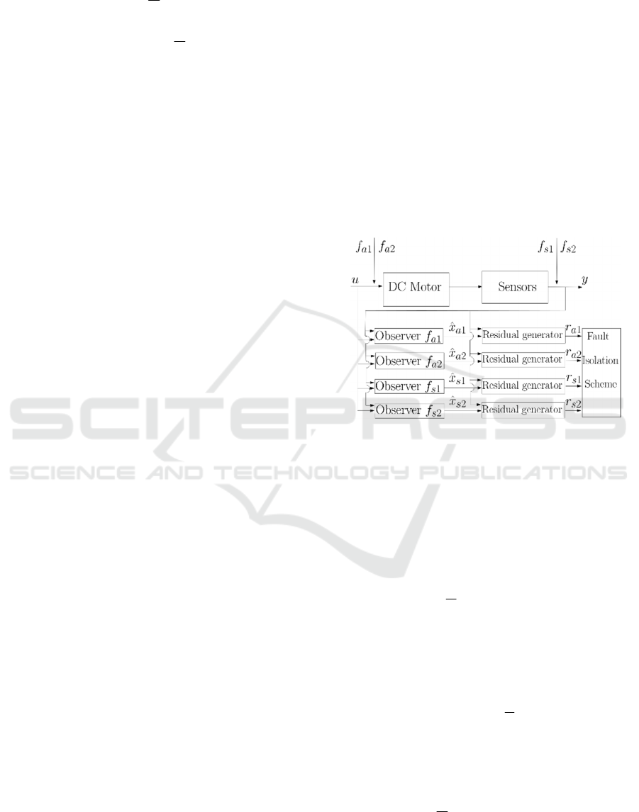
scheme on the base of residual signals (fig. 1). Let’s
analyze motor behavior under actuator and sensor
faults.
Figure 1: Fault detection and isolation scheme.
3.1 Torque Fault Detection
Some unaccounted force acting on the rotation of
mechanical parts causes torque fault. Error dynamic
takes the form
(8)
where
is an external force momentum acting
on rotor.
Consider condition 1:
(9)
It holds if we choose
=
:
(10)
1
2
1
2
1
0
,
1
0
10
,
01
a
a
s
s
f
J
xAxBu
f
L
f
yCx
f
=++
=+
ˆˆ ˆ
(),
ˆˆ
,
x
Ax Bu K y y
yCx
=++ −
=
ˆˆ ˆ
() ,r yyCxx CeyCx=−= − = =−
(),
,
ii
eAKCelf
rCe
=− +
=
[]
11
11
() ,
1
00,
aa
T
a
eAKCelf
ll
J
=− +
==
[]
111
11
331
1
()
;( ) 1
0( )
aa
akl
rank l A KC l rank
J
akl
−
−= =
−
111
1
()
1
00
akl
rank
J
−
=
Adaptive Fault Detection and Isolation for DC Motor Input and Sensors
705

Consider condition 2. Characteristic polynomial
of error model (8) takes the form:
(11)
where s is a complex variable,
(12)
Characteristic polynomial doesn’t depend on
,
because of
=
and
=
. So we
can define
=0. One can choose positive n, m to
provide desired observer behaviour and complete K
calculation by solution of equations (12) with respect
to the k
1
, k
4
with known k
2
, k
3
and n, m chosen by the
designer.
Condition 3 is satisfied because we have only one
fault direction vector.
3.2 Voltage Fault Detection
A voltage fault occurs due to some failure in
electronic circuits and disturbances of input voltage
(for example, the crash of the transistor in motor
driver or influence of powerful non-stationary
external magnetic field). Error dynamic takes the
form
(13)
where f
a2
is an additive voltage applied to the
motor input.
Consider condition 1:
(14)
It holds if we choose k
2
= a
2
:
(15)
Consider condition 2. Characteristic polynomial
of error model (13) is the same as in for force fault
case (12). It doesn’t depend on k
3
because all terms
with k
3
are rejected due to k
2
= a
2
. So we can define
k
3
= 0. In the same way as in previous subsection one
can choose positive n, m to provide desired observer
behaviour by pole placement procedure and complete
K calculation by solution of equations (12) with
respect to the k
1
, k
4
.
Condition 3 holds because residual directions l
a1
and l
a2
are orthogonal.
3.3 Velocity Sensor Fault Detection
This fault occurs due to mechanical or electronic
failure in velocity sensor or its data channels.
Multiply or stuck measurement value are the most
common types of the failures. Taking into account
(4), error dynamic takes the form
(16)
where f
s1
is velocity sensor fault signal.
Residual directions l
a1
and l
a2
are basis vectors in
two dimensional residual space. Therefore, it is
impossible to build linearly independent l
s1
with
respect to l
a1
and l
a2
in the same time. Let us choose
the following residual direction
=
=
11
. If the residual signal is along this direction,
then this fault will be more likely. Moreover, we can
provide mutual isolability with one of actuator faults.
Consider condition 1:
(17)
It is impossible to design such k
2
and k
4
that the
columns will be linearly dependent like in actuator
faults case because one of observer poles will be
equal to zero. Let rows will be linearly dependent to
satisfy the condition. Therefore:
(18)
One can find k
2
as a solution of (18):
(19)
The last coefficient k
4
is chosen to satisfy
condition 2 with use of characteristic polynomial
(12).
It is impossible to provide condition 3 for all
simultaneous faults, but proposed scheme allows to
isolate a velocity sensor fault with one of actuator
faults.
2
1
det( ( )) ,
a
p
sI A KC s ms n=−−=++
114 4
14 14 14 14 23 23 32 23
,
.
mk a a k
nkaaakkakkkakakaa
=−−+
=−+−−++−
[]
22
22
() ,
1
00,
aa
T
a
eAKCelf
ll
L
=− +
==
[]
222
22
442
0( )
;( ) 1
1
()
aa
akl
rank l A KC l rank
akl
L
−
−= =
−
442
00
1
1
()
rank
akl
L
=
−
11
1
1
3
() ,
1
,
0
s
s
s
eAKCelf
k
lKC
k
=− +
==
[]
1111223
11
3331443
()( )
;( ) 1
()()
ss
kakkakk
rank l A KC l rank
kakkakk
−+−
−= =
−+−
111 2 23
1
3331443
()( )
()()
akk a kk
k
kakkakk
−+−
=
−+−
22
113 2 3 31 413 13 4
2
2
3
akk ak ak akk kkk
k
k
+−− +
=
ICINCO 2022 - 19th International Conference on Informatics in Control, Automation and Robotics
706
3.4 Current Sensor Fault Detection
Reasons for current sensor faults are the same as for
velocity sensor. Error dynamic is described by
equations
(20)
where f
s2
is a velocity sensor fault signal. Choose fault
direction as
=
=
21
. This direction
is isolable from one of previous faults (condition 3 is
partially satisfied). Consider condition 1:
(21)
Similarly to previous subsection:
(22)
Therefore, k
3
is a solution of (22):
(23)
The last coefficient k
1
is chosen to satisfy
condition 2 with use of the characteristic polynomial
(12).
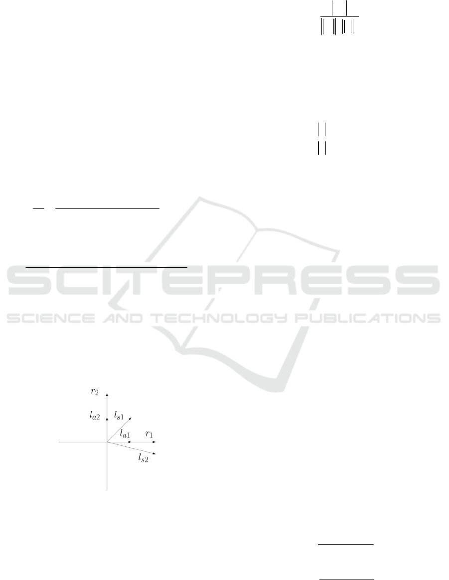
3.5 Fault Isolation Scheme
Faults directions in residual space are illustrated in
figure 2.
Figure 2: Fault directions in residual space.
However, it is impossible to provide explicit
separation of all simultaneous faults because two of
its directions define basis of two dimensional residual
space. But we can propose a scheme that allows faults
detection and isolation with the use of directional
relationship similarly to (Chen et all, 1996).
Introduce directional relationship Z between
residual vector r and fault direction l
i
2
2
.
T
i
i
T
i
lr
С
lr
=
(24)
Coefficient Z
i
denotes normalized value of
residual projection on the i-th fault direction. If Z
i
>
Z
j
then fault i is more likely then j. The most likely
fault corresponds to max(
), i = {
,
,
,
}.
Robustness with respect to the noises can be
provided by use of threshold:
,
0,
,
,
r if r Threshold
r
if r Threshold
≥
=
<
(25)
Problem of insensitivity to parametric
uncertainties can be overcome with the use of
identification algorithms. However, observer matrix
becomes depending on estimates of plant parameters
to perform all necessary detection conditions.
It should be noted, condition 3 is not satisfied for
all possible mutual faults. Hence, proposed scheme
may lead to isolation errors in cases of multiple faults.
For example, two simultaneous actuator failures can
cause increasing of the residual vector in sensor fault
direction. However, such situation is unlikely in
practice and detection algorithm remains its
performance.
4 ADAPTIVE MODIFICATION
Combine proposed method with the method of
dynamic regressor extension and mixing (DREM)
(Aranovskiy, Bobtsov, Ortega & Pyrkin, 2016;
Aranovskiy, Belov, Ortega, Barabanov & Bobtsov,
2019) for online estimation of parameters to ensure
FDI operability under uncertainties and non-
stationarity.
4.1 Plant Parameterization
It is necessary to transform (3) to the autoregressive
model for use of DREM. Rewrite plant (3) in transfer
function representation. Transfer functions with
current and velocity outputs take the form:
12
2
34
() ,
i
s
Ws
ss
ωω
ωω
+
=
++
(26)
5
2
34
() ,Ws
ss
ω
ω
ωω
=
++
(27)
22
2
2
4
() ,
0
,
1
s
s
s
eAKCelf
k
lKC
k
=− +
==
[]
2112224
22
4332444
()( )
;( ) 1
()()
ss
kakkakk
rank l A KC l rank
kakkakk
−+−
−= =
−+−
2112224
4332444
()( )
()()
kakkakk
kakkakk
−+−
=
−+−
22
32 424 124 24 124
3
2
2
ak akk akk ak kkk
k
k
+−−+
=
Adaptive Fault Detection and Isolation for DC Motor Input and Sensors
707

where
1
1
,
L
ω
=
2
,
f
k
L
J
ω
=
3
,
f
Lk RJ
LJ
ω
+
=
4
,
fbm
Rk k k
LJ
φ
ω
+
=
5
.
m
k
k
L
J
φ
=
There are unmeasured derivatives of i(t) and ω(t)
that prevents transformation to the autoregressive
model.
Rewrite (26), (27) as differential equations:
2
341 2
2
341 2
() () () () (),
() () () () (),
s
it sit it sut ut
s
tsititsutut
ωωω ω
ωω ωω ω
=− − + +
=− − + +
(28)
Apply second order stable linear filter with
characteristic polynomial
()=
+2+1 to
the left and right parts of (28) according to Ioannou &
Sun (2012):
2
3
41 2
2
3
41 2
,
() () () () ()
,
() () () () ()
s
ss
iiiuu
sssss
s
s
s
iiuu
s
sss s
ω
ωω ω
ωω ω
ω
ω
=− − + +
ΛΛΛΛΛ
=− − + +
ΛΛΛΛΛ
(29)
Coefficients λ
0
, λ
1
do not affect convergence time,
but appropriate choice allows to filter measurement
noises.
Equations (29) can be represented in desired form
with measured signals:
,
,
T
fi i i
T
f
yq
yq
ωωω
η
η
=
=
(30)
where
2
10 0
22
1
2
,,
fi f
ss
yiy
ss ss
ω
ω
λλ λλ
==
++ ++
110
2
0
2
1
;;
T
i
s
qii
ss ss
λλ λλ
=− −
++ ++
01
22
10
1
;
s
uu
ss ss
λλ λλ
−=
++ ++
11 1 1
1234
;;; ,
ii i i
qqqq
=
[
]
[
]
1234 1234
;;; ;;; ,
T
i
ηω ηωω η ηω
η
==
(31)
10 1
22
0
1
(); ;()
T
s
qt
ss s
t
s
ω
ωω
λλ λλ
=− −
++ ++
10
11 1
123
2
1
() ; ; ,ut q q q
ss
ωω ω
λλ
=
++
[
]
[
]
534 534
;; ;; .
T
ω
ηηηωωω
η
==
and
η
i
,η
ω
are transfer function unknown parameters
vectors to be identified.
4.2 Identification Algorithm
Let us use DREM method for DC motor parameters
online identification (Aranovskiy et all, 2016). This
approach provides independent estimation of plant
parameters and convergence speed tuning.
According to Margun et all (2021) and Nguev et
all (2021), apply different stable linear filters to (30)
2
22
33 44
22 3
2
3
22
,
,,
,,
TT
fi
TT
fi
T
f
ii
fi
T
ff
ii
yyqq
ss
yq yq
yq yq
ωωωω
η
η
ηη
λ
η
λλ
λ
η
==
++
==
=
=
=
(32)
where λ
i
are unique positive constants. Algorithm
for λ
i
selection doesn’t exists. However, there are
following heuristics can be used: large differences
between filter’s parameters decrease convergence
time; too large or small λ
i
can sufficiently increase
computation complexity; it is good practice to choose
filters parameters that are ten times different.
Obtain an extended system which includes (30)
and (32) in matrix representation:
,,
iii
YQY Q
ωωω
η
η
==
(33)
where
=
;
;
;
,
=
;
;
Multiply both equations (33) from the left by
adjoint matrix of
Q
i
,Q
ω
respectively. Yields
{
}
{}
,
,
iii
diag
diag
ωωω
ξϕ
η
ξϕ
η
=
=
(34)
where
φ
i
and
φ
ω
are determinants of matrices
Q
i
and
Q
ω
respectively.
Multiplication of (33) by adjoint matrix provides
independent regressors for parameters estimation
(one separate regressor for each unknown plant
parameter). This allows to design an independent
scalar identification algorithm for each parameter
similar to the classical gradient descent approach with
simplified tuning and fast convergence:
()
2
,
ˆˆ
nn nnn т
ηξϕϕηγ
−=
(35)
ICINCO 2022 - 19th International Conference on Informatics in Control, Automation and Robotics
708
where
γ
n
>0 is a design parameter that allow to tune
the convergence speed, ̂
is an estimate of the
corresponding parameter n. Separate parameters
identification and convergence speed tuning are main
advantages of DREM. One parameter change doesn’t
influence on others parameters estimates. This fact
provides the robustness of fault isolation in
comparison with gradient descent and least squares
approaches.
4.3 Adaptive Fault Detection and
Isolation
To ensure the adaptability of fault isolation scheme it
is necessary to combine it with a parameters
identification algorithm. It should be noted, that the
observer matrices depend on the identifier outputs.
This leads to the fact that during transient processes
the values of the observer matrices will have
significant errors in comparison with the desired
values. This may lead to false faults detections. We
need to update values of observers matrices only after
the end of identification algorithm transients to
overcome this drawback. It can be performed with the
use of sliding window:
(
̅
(
)
̂
(
)
)
∀,
(36)
where ̅ =
(
)
/ is a mean value on
period
(
;
)
,
is a threshold value.
Moreover, detection scheme should be insensitive
to the noises, small disturbances and deviations. This
problem can be solved with a residual deadzone
condition:
∆
=0
(37)
5 SIMULATION RESULTS
Consider motor with following plant
Observers matrices
K
a1
,K
a2
,K
s1
,K
s2
are updated
after parameters estimation transient time. Their
initial values can be calculated for nominal plant.
Characteristic polynomial for plants (26), (27)
parameterization is ()=
+2+1.
Parameters of DREM filters are chosen as follows:
for current output transfer function
=0.1,
=1,
= 10; for velocity output transfer function
=
0.1,
=1. Threshold values are
= 0.05,
=0.1, all values equal to one, =
10
(
0.1
)
+sin
(
)
to satisfy the persistent
excitation condition.
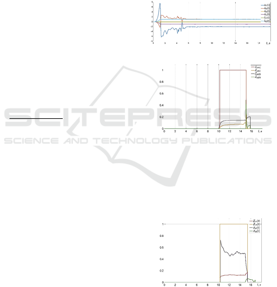
Identification algorithm results are shown figure
3. Parameters estimate converges to the true value of
six seconds. Observers matrices tend to the following
values:
Figure 4 illustrates fault isolation algorithm
output during external momentum acting on rotor
shaft from 10 to 15 seconds. Fault signal is a constant
that increases velocity. The largest value of
directional relationships
C
a1
corresponds to the
failure.
Figure 3: Plant parameters identification.
Figure 4: Directional relationships with force momentum
fault from 10 to 15 seconds.
The case of voltage fault is illustrated in figure 5.
The fault signal is an additional voltage applied to the
motor input. The directional relationship allows to
isolate this fault.
The case of sensor fault is illustrated in figure 6.
The fault is a current sensor zero shift that may be
caused by corruption of information bites. Proposed
scheme allows to isolate this sensor fault.
Figure 5: Directional relationships with voltage fault from
10 to 15 seconds.
Adaptive Fault Detection and Isolation for DC Motor Input and Sensors
709
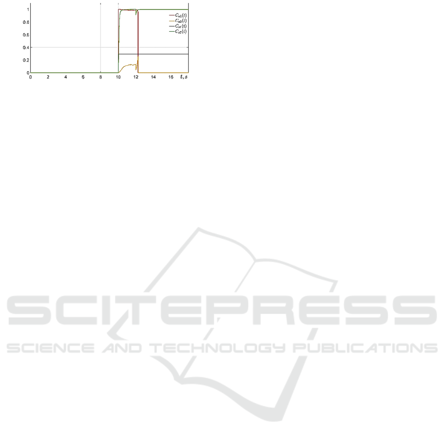
Figure 6: Directional relationships with current sensor fault
since 10 seconds.
6 CONCLUSION
Actuator and sensor adaptive fault detection and
isolation scheme for direct current motor is proposed.
The motor is assumed to be equipped with velocity
and current sensors. Detection algorithm is observer
based. Isolation scheme uses directional relationship
between residual and fault directions.
Adaptability is provided by DREM approach.
Proposed solution allows to isolate torque fault, input
voltage fault, velocity sensor fault and current sensor
fault. Simplicity of observers and residual generators
synthesis and its trivial computation are advantages
of the scheme.
Robustness with respect to the noise is obtained
by use of threshold. Insensitivity to uncertainties is
provided by the DREM approach and switching
techniques for the tracking of estimation end.
Simulation results confirm the effectiveness of the
proposed approach.
ACKNOWLEDGEMENTS
The work is supported by the Russian Science
Foundation grant (project 19-19-00403).
REFERENCES
Wunnenberg, J. (1990). Observer-based Fault Detection in
Dynamic Systems, VDI Verlag, 127 p.
Chen, J., Patton, R. J. (1999). Robust Model-Based Fault
Diagnosis for Dynamic Systems, Kluwer
Ray, A., Luck, R. (1991). An introduction to sensor signal
validation in redundant measurement systems, Control
Systems, IEEE. 11., pp. 44 - 49.
Patton, R. J., Chen, J. (1997). Observer-based fault
detection and isolation: Robustness and applications,
Control Engineering Practice, Volume 5, Issue 5, pp.
671-682.
Chung, W. H., Speyer, J. L. (1998). A game theoretic fault
detection filter, IEEE Transactions on Automatic
Control, vol. 43, no. 2, pp. 143-161.
Chen, J., Patton, R., Zhang, H.-Y. (1996). Design of
unknown input observers and robust fault detection
filters. International Journal of Control, 63, pp. 85-105.
10.1080/00207179608921833.
Isermann, R. (1997). Supervision, fault-detection and fault-
diagnosis methods, An introduction, Control
Engineering Practice, Volume 5, Issue 5, pp. 639-652.
Santos, L.I., Palhares, R., D’Angelo, M., Endes, J.B.,
Veloso, R., Ekel, P. (2018). A New Scheme for Fault
Detection and Classification Applied to DC Motor, pp.
327-345. 10.5540/tema.2018.019.02.0327.
Adouni, A., Abid, A., Sbita, L. (2016). A DC motor fault
detection, isolation and identification based on a new
architecture Artificial Neural Network, 5th
International Conference on Systems and Control
(ICSC), pp. 294-299.
Isermann, R. (2006). Fault detection and diagnosis of DC
motor drives. In: Fault-Diagnosis Systems. Springer,
Berlin, Heidelberg.
Margun, A., Kremlev, A., Vlasov, S. (2021). DREM based
DC motor components fault detection and isolation,
29th Mediterranean Conference on Control and
Automation, pp. 1052 - 1057.
Nguyen, T.K., Vlasov, S.M., Margun, A.A., Kirsanova,
A.S. (2021). Identification of DC motor parameters
using method of dynamic regressor extension and
mixing, 29th Mediterranean Conference on Control and
Automation, pp. 718 - 722.
Clark, R. N. (1979). The dedicated observer approach to
instrument failure detection, 18th IEEE Conference on
Decision and Control including the Symposium on
Adaptive Processes, pp. 237-241. Academic
Publishers, Boston, MA,U.S.A. 354 p .
Aranovskiy, S., Bobtsov, A., Ortega, R., Pyrkin, A. (2016).
Parameters estimation via dynamic regressor extension
and mixing, 2016 American Control Conference
(ACC), pp. 6971-6976.
Aranovskiy, S., Belov, A., Ortega, R., Barabanov, N.,
Bobtsov, A. (2019). Parameter identification of linear
time-invariant systems using dynamic regressor
extension and mixing, International Journal of Adaptive
Control and Signal Processing, 33(6), pp. 1016–1030.
Ioannou, P., Sun, J. (2012). Robust Adaptive Control.
Dover Books on Electrical Engineering, 821 p.
ICINCO 2022 - 19th International Conference on Informatics in Control, Automation and Robotics
710
