Improving Car Detection from Aerial Footage with Elevation

Information and Markov Random Fields

Kevin Qiu

, Dimitri Bulatov

and Lukas Lucks

Fraunhofer IOSB Ettlingen, Gutleuthaus Str. 1, 76275 Ettlingen, Germany

Keywords:

DeepLab, Machine Learning, Remote Sensing, Markov Random Fields.

Abstract:

Convolutional neural networks are often trained on RGB images because it is standard practice to use transfer

learning using a pre-trained model. Satellite and aerial imagery, however, usually have additional bands, such

as infrared or elevation channels. Especially when it comes to detection of small objects, like cars, this addi-

tional information could provide a signiﬁcant beneﬁt. We developed a semantic segmentation model trained on

the combined optical and elevation data. Moreover, a post-processing routine using Markov Random Fields

was developed and compared to a sequence of pixel-wise and object-wise ﬁltering steps. The models are

evaluated on the Potsdam dataset on the pixel and object-based level, whereby accuracies around 90% were

obtained.

1 INTRODUCTION

Vehicle detection in combined large-scale airborne

data has a wide range of applications. For improved

city planning, trafﬁc ﬂow estimation is essential. Also

for ecological sciences, it is helpful to know the av-

erage number of vehicles on the main roads, includ-

ing their velocities (Leitloff et al., 2014). In mili-

tary applications, vehicles may mean both targets and

threats (Gleason et al., 2011). Finally, for the applica-

tion of virtual tourism, situational awareness may be

increased if the so-called inpainting is applied to re-

ﬁll the data from the temporary objects, like vehicles

(Leberl et al., 2007; Kottler et al., 2016). A success-

ful inpainting, which is our main motivation for this

paper, implies the necessity to detect every single ve-

hicle, including those partly occluded and away from

roads (Schilling et al., 2018b).

However, variations of scale, orientation, illumi-

nation, as well as the complexity of background repre-

sent the main challenges for vehicle detection. One of

the possibilities to reduce these effects is using mod-

ern Deep Learning architectures such as (Chen et al.,

2018), preferably trained with large data-bases, such

as ImageNet (Russakovsky et al., 2015), and relying

on sophisticated data augmentation modules, which

https://orcid.org/0000-0003-1512-4260

https://orcid.org/0000-0002-0560-2591

https://orcid.org/0000-0003-2961-3452

take into account to the problems mentioned above.

For single vehicle extraction, one can either use in-

stance segmentation networks, such as (Mo and Yan,

2020), but we omit them since they need even more

parameters to be determined, and thus, more train-

ing time is expected. Instead, we will concentrate

on post-processing routines using Markov Random

Fields. Their big advantage is that only a few pa-

rameters are needed to model, to a major part, quite

a broad spectrum of situations. From the pixel-wise

prediction we will impose soft non-local constraints

on pixel neighborhoods to improve detection results

on pixel and object level.

Another possibility to reduce at least the illumi-

nation variation is to use elevation data, which may

be acquired from optical images using the state-of-

the-art photogrammetric procedures (Snavely et al.,

2006). From dense point clouds, a digital surface

model can be created (Bulatov et al., 2014). There-

after, we can subtract from it the ground model and

obtain the relative elevation, in which cars appear as

standardized objects with respect to their elevation.

Thus, in this paper, we will assume the availability

of a high-quality relative elevation image in the same

coordinate system as the optical image. Still, several

questions will arise. First of all, what happens to the

moving vehicle, which are usually not modeled well

in photogrammetric point clouds. Second, how and

at which stage should the elevation data be consid-

ered to achieve the best results. If it is considered at

112

Qiu, K., Bulatov, D. and Lucks, L.

Improving Car Detection from Aerial Footage with Elevation Information and Markov Random Fields.

DOI: 10.5220/0011335900003289

In Proceedings of the 19th International Conference on Signal Processing and Multimedia Applications (SIGMAP 2022), pages 112-119

ISBN: 978-989-758-591-3; ISSN: 2184-9471

the beginning, then the problem of scarcity of training

data could become an obstacle. Otherwise, if used for

post-processing only, it is questionable whether insuf-

ﬁciencies committed at the beginning, such as missed

detections, can ever be corrected. Third, one could

argue that elevation, obtained from the optical data,

does not represent a new source of information, and

the beneﬁt such elevation data can bring about is lim-

ited.

In order to be able to answer these questions, we

decided to develop a multi-branch architecture con-

sisting of a standard RGB branch and an improvised

second branch that contains elevation data and/or

some additional data typical for remote sensing. Us-

ing only one hyper-parameter for weighting, we can

compare predictions based on RGB data only with

those obtained by the improvised branch. As a second

contribution, we will apply the post-processing result

using MRFs. Their sophisticated priors ensure that

vehicles may or may not have a standardized height.

The fact that we are working on a two-class prob-

lem guarantees a fast convergence of a simple move-

making energy minimization method. To explore the

effect of MRFs, it is often helpful to perform train-

ing and prediction on rather low-quality data, such as

decay on resolution. The experiments are carried out

on the well-known Potsdam dataset because the avail-

able, though not always perfect ground truth provide

a solid basis for evaluations.

We organize this article into a summary of pre-

vious works in Section 2, followed by description of

our methodology in Section 3, results (Section 4) and

conclusions (Section 5).

2 PREVIOUS WORK

The methodology on vehicle detection in remote sens-

ing data can be subdivided into conventional and

deep-learning-based methods. In the ﬁrst category,

detection can be carried out explicitly, leaving some

parts of the scene unconsidered (Zhao and Neva-

tia, 2003; Cao et al., 2019). Model-driven identi-

ﬁcation, sometimes denoted as segmentation (Bula-

tov and Schilling, 2016), has as its primary goal to

achieve the hightest possible recall value while the

precision is supposed to be improved after application

of the method of machine learning (Schilling et al.,

2018a; Madhogaria et al., 2015). For example, in

(Schilling et al., 2018a), stripes formed from almost

parallel line segments detected in the optical and el-

evation data were identiﬁed as the best tool to cre-

ate hypotheses. After this, a feature set over different

sensor data is used to perform classiﬁcation and sin-

gle vehicle extraction. The next level of abstraction

is to use generic feature extractors such as histograms

of orientated gradients (HOG), scale-invariant feature

transform, or others for hypotheses generation, and

then to build a higher-level object description to sub-

ject these feature-rich instances to a classiﬁer, like

AdaBoost or support vector machines (SVM) (Leit-

loff et al., 2014; Chen et al., 2015; Madhogaria et al.,

2015). The approach of (Yao et al., 2011) works in a

similar way, but it relies on 3D points.

We concentrate here more on deep-learning-based

methods because they became state of the art in many

tasks of object detection and semantic segmentation

due to their universality. Probably, the ﬁrst approach

developed on vehicle detection from remote sensing

data using CNN techniques was that of (Chen et al.,

2014) who extracted multi-scale features and com-

bined it with a modiﬁed sliding window technique.

Furthermore, (Ammour et al., 2017) proposed extrac-

tion of deep features from segments and classiﬁca-

tion of these features using SVM. The authors have

built on the progress in fully-convolutional networks

and residual learning to perform accurate segmenta-

tion of object borders. In their semantic boundary-

aware multitask learning network, detection and seg-

mentation of vehicle instances were trained simulta-

neously. Approximately at the same time, (Tayara

et al., 2017) accomplished detection of vehicles using

a pyramid-based network with convolutional down-

sampling as well as deconvolutional upsampling lay-

ers. As for the combined optical and elevation-based

features, (Schilling et al., 2018b) designed a two-

branch CNN model. The branches were built after a

pre-trained pseudo-Siamese network allowed to com-

pute features from RGB channels and elevation chan-

nels, which were successively merged. There was

also a module for single vehicle extraction and hav-

ing the heat-map as input. Overall, progress made

on fully-convolutional networks, equipped either with

encoder-decoder structures, with skip connections or

atrous convolutions (Chen et al., 2018), nowadays

helps to overcome pooling artifacts within the state-

of-the-art land cover classiﬁcation pipelines, such as

(Volpi and Tuia, 2016; Liu et al., 2017). Therefrom,

obtaining the car class is a trivial operation, and a sin-

gle vehicle detection can be achieved by (Schilling

et al., 2018b), for instance. Two contributions (Tang

et al., 2017) and (Mo and Yan, 2020) rely on instance

segmentation. The hyper region proposal network

(Tang et al., 2017) aims at predicting all of the possi-

ble bounding boxes of vehicle-like objects with a high

recall rate. A cascade of boosted classiﬁers reduces

spurious detections by explicitly including them into

the loss function (hard negative example mining). In

Improving Car Detection from Aerial Footage with Elevation Information and Markov Random Fields

113

the work of (Chen et al., 2019), a modiﬁcation of

DeepLabV3 (Chen et al., 2018), aimed at recognizing

ﬁne-grained features, is proposed and the results are

post-processed using generalized Zero-shot learning.

Recognition of previously unseen vehicles takes place

using both latent attributes, obtained within a least

square minimization framework, and human-deﬁned

attributes. One of the newest trends in Computer Vi-

sion is to use generative adversarial techniques. It is,

therefore, not surprising that the authors of (Ji et al.,

2019) applied a super-resolution convolutional neu-

ral network to train the detection of vehicles in an

end-to-end manner. This was done by integrating the

loss based on target detection directly into the super-

resolution network. The features at different scales

were combined to generate the ﬁnest feature map for

the subsequent detection.

Finally, we refer to literature aiming at car detec-

tion using MRFs and CRFs. A comprehensive op-

timization pipeline (Madhogaria et al., 2015) uses a

message-passing-like algorithm with features stem-

ming from color values of neighboring pixels. In the

segment-based method of (Liu et al., 2017) for gen-

eral semantic segmentation, a high-order CRF was

introduced, encouraging pixels of the same segment

to belong to the same class. The results for the car

class are quite high (F-score exceeding 94%); how-

ever, the accuracy depends strongly on the segmenta-

tion method.

3 METHODOLOGY

Throughout this paper, we use non-capital bold let-

ters x, y for pixels and pixelwise states s, and capital

italic letters for images J, relative elevation data Z,

and image-wise states S.

3.1 Combined DeepLabV3+ Model

Since the conventional DeeplabV3+ model, denoted

as Deeplab from now on, is described in (Chen et al.,

2018), we restrict ourselves to mentioning some im-

portant characteristics that make up difference to

the proposed network, which is illustrated in Figure

1A. The backbone is ResNet101 (He et al., 2016).

The layers in Fig. 1A correspond to ResNet resid-

ual blocks. Similar to (Audebert et al., 2016), we

extended the architecture of Deeplab to accept six

input layers. Thus, the backbone is split into two

branches, where one branch processes the traditional

RGB image channels while the additional bands pro-

cess three more channels. For the dataset available

(see Section 4.1), these bands are the near-infrared

channel, the Normalized Differential Vegetation In-

dex (NDVI) channel, and the relative elevation. If

there are more than three additional bands, it is al-

ways possible to compute a PCA from these chan-

nels. The two branches are both initialized using the

pre-trained weights of ImageNet (Russakovsky et al.,

2015). Even though the pre-training was done on

RGB images, the earlier shallow levels of the net-

works are supposed to detect simple patterns, such as

edges and shapes, which was the reason to use pre-

trained weights for the additional branch, too. Also,

this fact motivated us to merge the features computed

for both as early as possible. At the ﬁrst layer of

Deeplab, we applied a convex combination.

F = αF

+ (1 − α)F

, 0 ≤ α ≤ 1 (1)

which means that, for example, setting α = 1 is equiv-

alent to the conventional method, while a symmetric

weighting of features F

J,H

will be used in this work,

that is α = 0.5.

We perform the standard modules on data aug-

mentation during training to reduce overﬁtting effects.

Even though we focus on car detection in this paper,

we wish to preserve our network so general as possi-

ble bearing in mind the over-reaching goal of scene

representation using multi-modal input data. There-

fore all six available classes of the dataset are used for

training, and not two-class classiﬁcation. The classes

include cas, tree, impervious surfaces, low vegetation,

clutter and building. The batch size is set to 8, the

output stride of Deeplab is set to 16, and Adamw opti-

mizer (Loshchilov and Hutter, 2017) was used to min-

imize the cross entropy as our loss function.

3.2 MRF

A Markov Random Field is a statistical model con-

sisting of an undirected graph that satisﬁes the lo-

cal Markov properties. The nodes of the graph are

random variables (x) whose state s is only depen-

dent on that of the neighbors. These neighbors, de-

noted by N, are represented by the graph edges. In

our case, the graph is a pixel grid, where the nodes

represent the pixels, and each pixel is connected to

its four direct neighbors. Each node x has only two

states: car (s

= 1) and non-car (s

= 0). We denote

by P(J) = P(J

= 1) the value softmax probability

that x is a car pixel, which is the output of our neu-

ral network. Since the elevation channel incorporates

important information about absolute values typical

for cars, we also deﬁne the likelihood of a car having

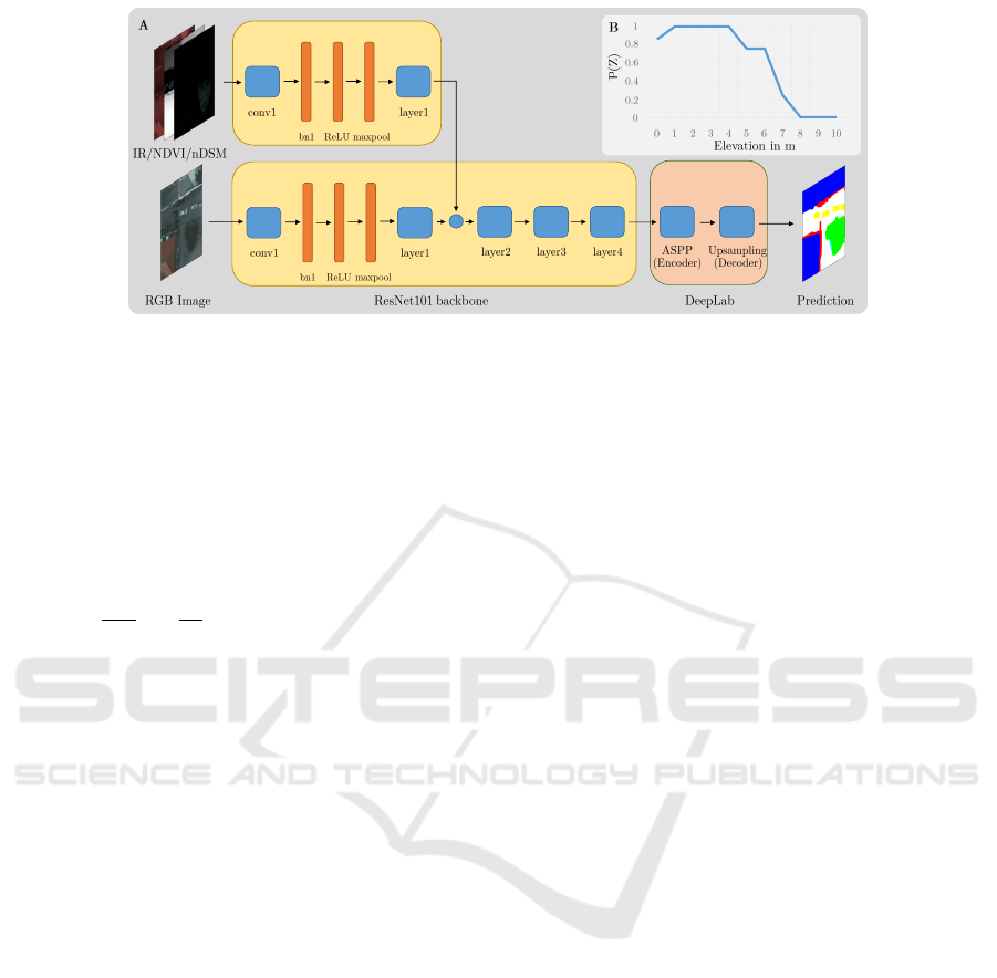
a certain height as P(Z), shown in Fig. 1, B. Since

moving cars do not have salient relative elevations,

we set P(Z = 0) = 0.85. Elevation over 4 m is quite

SIGMAP 2022 - 19th International Conference on Signal Processing and Multimedia Applications

114

unlikely for a car, and here is where the function P(Z)

experiences a steep decay.

Overall, the cost function is deﬁned as:

E(s) =

∑

) +

∑

x,y∈N

, s

)

→ min (2)

The data C

) and smoothness C

, s

) term

across all graph nodes are summed up and minimized

to solve for the unknown S = {s

|x ∈ J}. The data

term includes the network-induced detection proba-

bility P

and the height probability P

= 1) = − log [βP

J∩Z

+ (1 − β)P

J∪Z

]. (3)

The term in square brackets in (3) is the combined

probability P

J∩Z

= P(J) · P(Z), since we can assume

P(J) and P(Z) to be statistically independent, and

P(J ∪Z) = P(J)+P(Z)−P(J)·P(Z). For most cases,

we want both probabilities to be high. However, in

some situations, we would be happy with a logical

“or”. For example, if a car is parked atop a roof, we

want to grant it an opportunity to be detected. Ac-

cording to fuzzy-logical concepts, we weight both ob-

servations with a scalar β, which usually lies between

0.5 and 1. We note that C

= 0) is the negative

logarithm of the complementary to (3) probability.

The smoothing term in (2) is deﬁned as:







0, if s

= s

λ · exp



−

∆

−

∆



, otherwise.

(4)

As usually, it penalizes neighbored pixels x and y if

they are labeled differently. The weight of penaliza-

tion depends inversely on how different the elevation

and color value of x and y. We denote by ∆Z the dif-

ference of elevations Z(x) − Z(y) and by ∆J the norm

of the difference in the CIELAB color space (Tomi-

naga, 1992). CIELAB is known to reﬂect human per-

ception of colors, which appear practically incorre-

lated in this representation. In order to balance the

data and smoothness terms, the parameter λ has to be

chosen carefully. We worked with the value 50 while

the choice σ

and σ

was 1 and 5, respectively.

Minimization of (2) takes place using the Alpha-

expansion method of (Boykov et al., 2001). The fact

that we only have two labels for our MRF and also

due to the sub-modularity of our smoothness function

in (4) allows convergence to the global minimum

after only one iteration.

4 EXPERIMENTS

4.1 Potsdam Dataset

The Potsdam dataset (Rottensteiner et al., 2014) is

the ISPRS benchmark consisting of 14 patches with

6000 × 6000 pixels and a resolution of 5 cm. The

resulting area of approximately 1.26 km

contained

3820 vehicles. For all patches, there was image and

elevation data available. Besides, the dataset has a full

reference ground truth for the six land cover classes

and also a reference where the boundaries of the ob-

jects are eroded by a circular disc of three pixel ra-

dius. The full reference ground truth is used, and all

six classes are trained. The training data is kept at its

original resolution of 5cm and cropped into patches

of 512 × 512 pixels. To further explore the effect of

MRFs, we considered an older model allowing only to

differentiate between classes vehicle and background.

This model was trained with a standard DeepLab, us-

ing optical data only, but on the eroded reference data

and a reduced resolution of 10cm. There was also

no overlap between the 256 × 256 pixels data patches

during inference, resulting in worse detection accu-

racy.

In order to guarantee the fairness of the compar-

ison, we applied some post-processing steps to the

older model. For example, since the eroded labels

were used to train this model, the car detections are

systematically eroded as well, inspiring us to apply

morphological dilation. Since the elevation data was

not considered during CNN computation, we also per-

formed object-wise ﬁltering. For every connected

component, the minimum median object height must

not exceed 10m while the minimum object size must

exceed 450 pixels, or 1.125m

. The minimum detec-

tion probability is set at 0.9.

4.2 Evaluation Strategy

Precision (p) and recall (r), as well as those uniﬁed

measures that can be formed from them, such Inter-

section over Union (IoU = (p

−1

+ r

−1

− 1)

−1

) and

F1-score, are the commonly used tools to assess the

accuracy of detection for small objects, like cars. We

decided to track these measures for both pixel-wise

and object-wise level because for many applications,

it would make a difference whether we correctly de-

tected half of the pixels of each car or 50% of the

cars completely and the other 50% not at all. Thus, to

decide whether a car has been detected on the object

level, we check whether there is a detection yielding

an IoU of at least 0.5. To do this, all cars and all con-

nected components formed by detections have been

Improving Car Detection from Aerial Footage with Elevation Information and Markov Random Fields

115

Figure 1: The architecture used in this article. bn and ASPP are abbreviations for Batch Normalization and Atrous Spatial

Pyramid Pooling, respectively (see (Chen et al., 2018)), while by layerX, we denote a residual block of ResNet. In the top

right image, the elevation-based likelihood P(Z) is depicted.

labeled, after which a 2D histogram has been com-

puted. From the entries of the 2D and two 1D his-

tograms, we compute the component-to-component

IoUs. Once we have found out which car has been

detected to a minimum threshold of IoU, which was

0.5, we can derive the object-based measures for pre-

cision, recall, IoU, and F1 score. Two latter ones are

denoted as IoU and F1 in Table 1.

4.3 Evaluation Results

4.3.1 Quantitative Assessment

As depicted in Table 1, the proposed network CNN

with only RGB data could obtain reasonably good re-

sults. We refrain from a more detailed comparison

with related approaches since, ﬁrst of all, all of them

use different training/validation splits on the Potsdam

dataset. Secondly, only a few of them, like (Schilling

et al., 2018b) report object-wise scores. Finally, for

the reasons of space, we do not report results of a

comprehensive ablation study. We found out that

equal weighing both branches (α = 0.5 in the new

model) yielded the best performance. As expected,

using the near-infrared channel and relative elevation

(α = 0.5) with the new model yielded the best per-

formance. Since the detection was performed using

images at the ﬁnest-possible resolution, the pixelwise

results improve signiﬁcantly neither after ﬁltering nor

after the application of MRFs despite our extensive

trials on algorithm parameters β, σ

, and σ

. The ob-

jectwise F1-measure, however, increases from 0.879

to 0.918 after ﬁltering.

Using RGB data only (α = 1.0), we obtain the

pixelwise F1-measure 0.890. After object-wise ﬁl-

tering, the F1-measure increases by 0.1% while the

object-wise F1-measure increases by 4.8% to 0.901.

The comparability results obtained using image data

only conﬁrms our apprehensions that the large param-

eter sets, obtained within a deep architecture from im-

ages only, already implicitly include the clues 3D data

may provide. However, one should take into account

some doubtful ground truth because, as the next sec-

tion 4.3.2 will show, the images were taken during

the winter, such that the cars are clearly visible un-

der the leaﬂess trees but are not annotated into the

images. This fact actually shows the positive side of

our method, namely, its ability to generalize but con-

tribute to commission errors in Table 1.

Besides, Table 1, together with the images com-

ing next, show that both models are able to outper-

form the older model, which was derived from the

sub-optimal training data. The older model can be

signiﬁcantly improved already using dilation and ﬁl-

tering (pixelwise F1 increases from 0.771 to 0.857).

Besides correcting the eroded training data, dilation

can also merge separated segments classiﬁed as ve-

hicles and improve the objectwise results (F1 im-

proves from 0.754 to 0.865). For this model, we have

achieved a signiﬁcant improvement using MRFs. It

is notable that a pixelwise improvement of MRFs is

bigger; however, the objectwise is lower, which has

to do with the fact that sometimes very narrow bor-

ders between very densely parked vehicles are added

to the car class, making the test on component-to-

component from Section 4.2 fail. This happens more

frequently in the case of dark cars upon similarly dark

soil where the color differences are lower. Occasion-

ally, false-positive detections, like trailers, containers,

or other rectangular-shaped objects, are falsely en-

larged by the MRF.

4.3.2 Qualitative Assessment

To gain an impression on differences in performance

of the considered methods, we refer to Figures 2 to 5.

SIGMAP 2022 - 19th International Conference on Signal Processing and Multimedia Applications

116

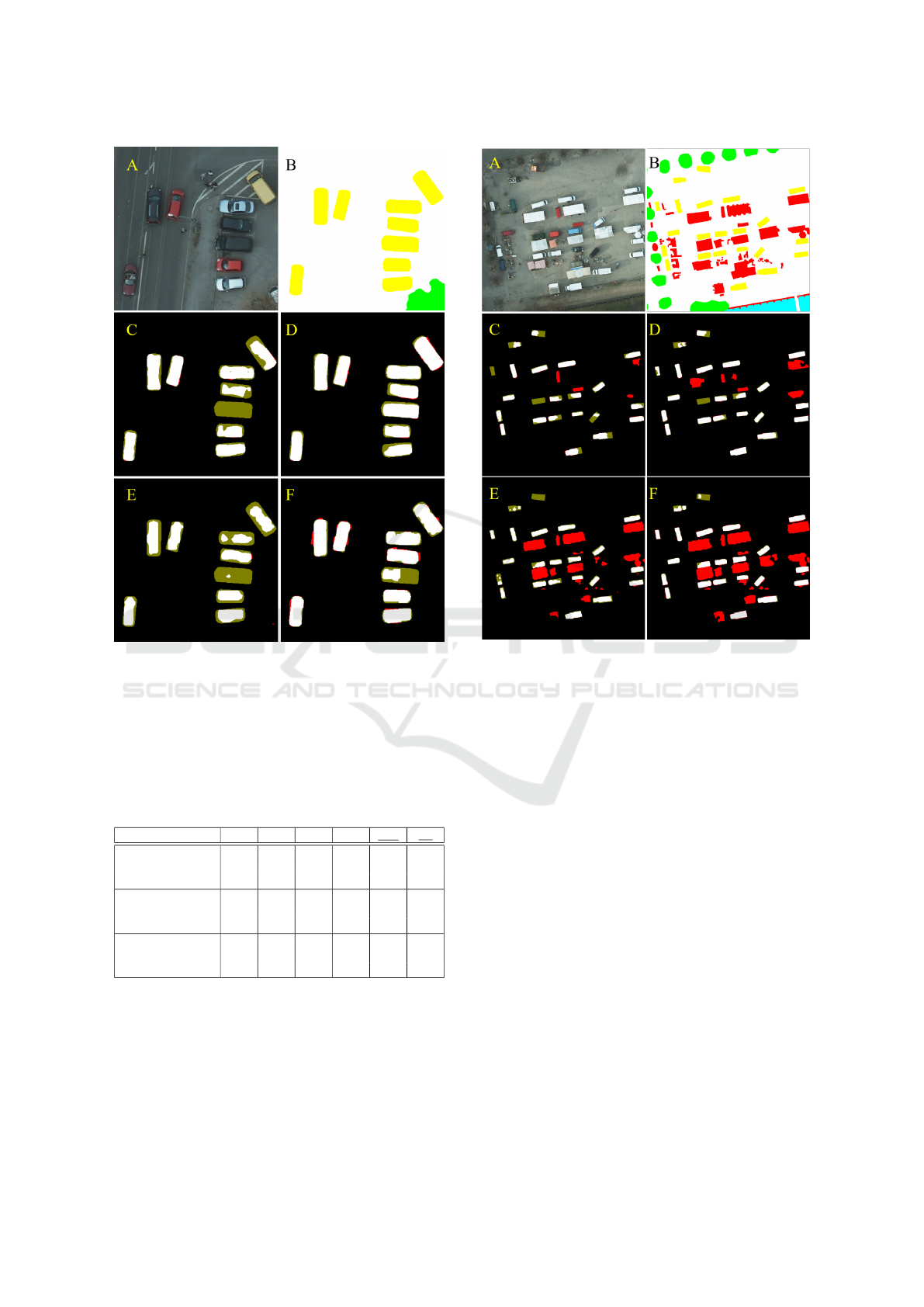
Figure 2: Qualitative results on detection of vehicles. A:

RGB image, B: ground truth, where cars are colored in yel-

low. C: The combined network (left α = 1 and D: α = 0.5),

whereby true positives, true negatives, false positives and

false negatives are colored in white, black, red and dark-

green color, respectively. E: the older model without and F:

with MRF-based post-processing.

Table 1: Quantitative comparison of three different models.

All results are given percents. Underlined variables denote

object-wise values.

Method r p IoU F1 IoU F1

Comb. α = 0.5 86.9 91.7 80.5 89.2 78.5 87.9

. . . +ﬁlter 86.7 91.9 80.6 89.2 84.8 91.8

. . . +MRF+ﬁlter 91.5 86.2 79.8 88.8 79.7 88.7

Comb. α = 1.0 90.1 88.0 80.2 89.0 74.4 85.3

. . . +ﬁlter 89.0 88.3 80.4 89.1 82.0 90.1

. . . +MRF+ﬁlter 91.7 84.1 78.1 87.7 69.8 82.2

Older model 66.2 92.4 62.8 77.1 60.5 75.4

. . . + dilate + ﬁlter 86.7 84.7 74.9 85.6 78.5 88.0

. . . + MRF + ﬁlter 85.4 86.8 75.6 86.1 78.0 87.6

In Figure 2, we see that a dark car could be retrieved

using elevation information. This is possible either

using the MRF inference (image E), boosting up the

data term, or the combined Deeplab (C), which uses,

among others, the elevation channel. At the same

time, ﬁltering does not produce new detections and

only suppresses the spurious ones. All other cars in

Figure 3: Another example on vehicle detection. See cap-

tion of Fig. 2 for further explanations. Note that the zoom

level differs from Fig. 2. The resolution remains at 5 cm.

the fragment have been detected, whereby we can see

that the images C and D resemble to their counterparts

on the right (E and F, respectively). Furthermore, Fig-

ure 3 shows an accumulation of market stands with

cars parked wildly among them, provoking a relative

confusion between the stands and the cars. Here we

see that the new model performs much better, since

it is also trained on the other classes of the Potsdam

dataset. However, one exception is a white car parked

too densely to the stands. Moreover, we see how the

MRFs, in general, improve the outlines in both bot-

tom images. In Figure 4, C, we can see how the

elevation information helps to detect confusion be-

tween the right-most car and the road lane while the

conﬁguration with α = 1 produces two spikes on the

sides (B). Apart from this, in Figures 4 and 5, we

see the difference between the application of dilation

and MRFs. While the dilation sometimes overshoots

the label boundary and is quite fuzzy at the edges,

which happens due to the upscaling from the lower

resolution, using MRFs improves the border of de-

tections, making them closer to the actual labels. Fi-

nally, the ground truth image of Figure 5 shows how

Improving Car Detection from Aerial Footage with Elevation Information and Markov Random Fields

117

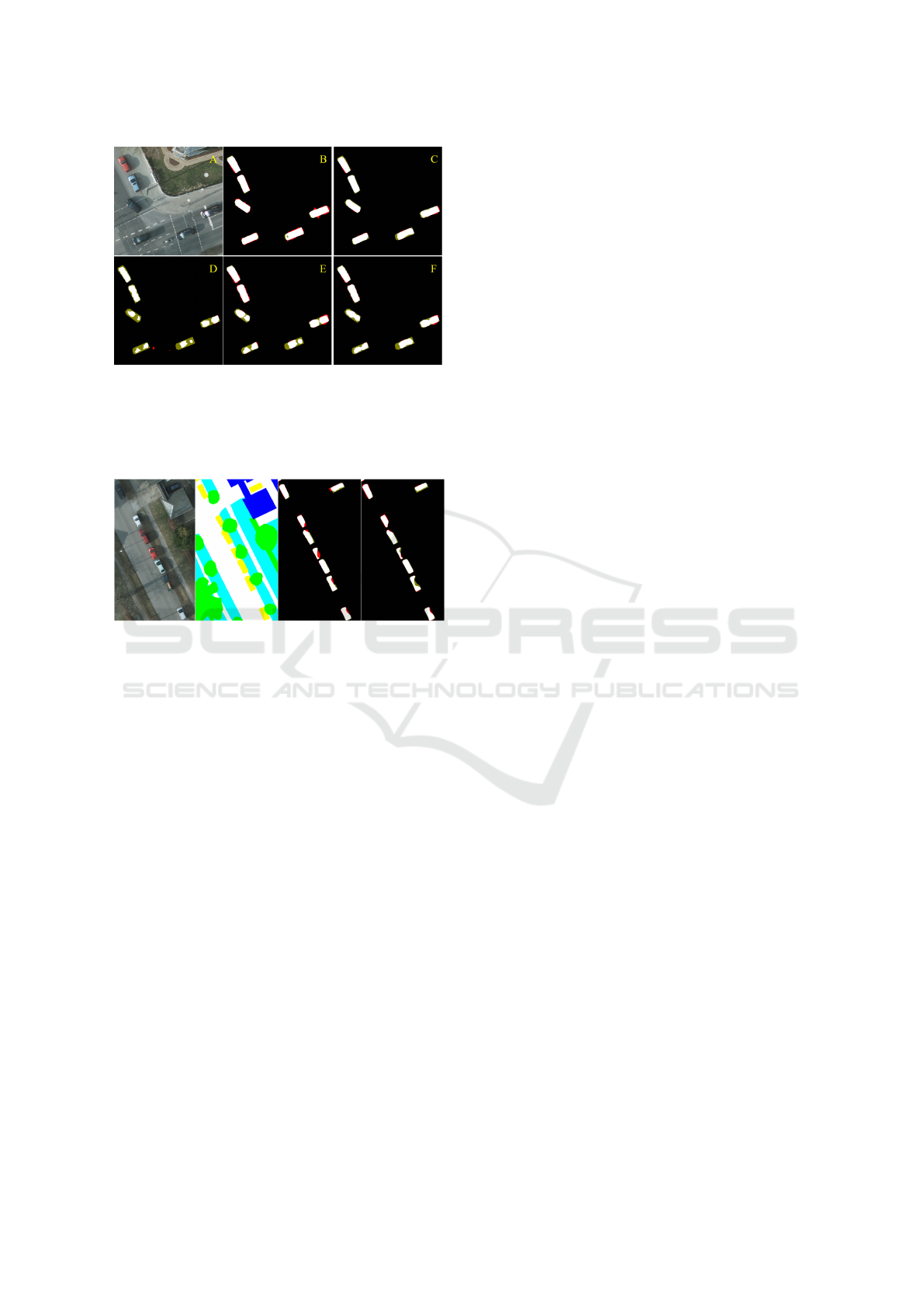
Figure 4: Example of a scene with moving cars. A: RGB

image as well as detections using the new pipeline (B:

α = 0 and C: α = 0). Bottom row: detections using the

old pipeline, result of dilation and ﬁltering as well as result

of MRFs following by ﬁltering. In images B-F, the color

choice is the same as in Figs. 2 and 3.

Figure 5: Exempliﬁcation of insufﬁciencies of the ground

truth data. From left to right: RGB image, ground truth, de-

tection result using the proposed network with α = 1, with-

out and with MRFs.

non-existent tree crowns in winter occlude cars and

slightly affect the result of MRFs. Since the new

DeepLab model is trained on all six classes, includ-

ing cars and trees, it is able to reproduce the occlu-

sion of cars by trees present in the ground truth. If

MRFs are then applied, the car detections tend to get

dilated to the entire car, even when that part is under-

neath a tree. This partialy explains why MRFs do not

improve in Table 1 for the newer DeepLab models.

This effect is not as pronounced on the older DeepLab

model, which was trained on just the car class. There,

even without MRFs, the model tends to detect the en-

tire car, even if underneath a tree because the model

generalized the car class.

5 CONCLUSION

We presented a method for vehicle detection from

high-resolution airborne data, whereby our innova-

tion to the DeepLabV3+ method (Chen et al., 2018)

is an additional branch relying on typical data for

remote sensing. Furthermore, an MRF-based work-

ﬂow has been implemented. We applied our data

to the benchmark data test and obtained encourag-

ing results. The accuracies obtained are slightly be-

low those cited in related works (Chen et al., 2019;

Schilling et al., 2018b), where only pixelwise predic-

tion was reported. However, our workﬂow is general

enough to be applied to the problem of land cover

classiﬁcation. For the most part, the false positives the

proposed method has produced were either different

moving objects, such as market stalls or trailers, or ar-

eas between densely parked cars with many shadows.

Fortunately, temporary objects of this kind are wel-

come to be removed during inpainting, which is our

main area of applications. We also experimented with

MRFs, which improved the results in the case of sub-

optimal training data. Here, MRFs are able to outper-

form simple object-wise ﬁltering methods based on

the objects height and size. In the future, we plan to

test the workﬂow for datasets of a coarser resolution,

followed by the application of inpainting methods.

REFERENCES

Ammour, N., Alhichri, H., Bazi, Y., Benjdira, B., Alajlan,

N., and Zuair, M. (2017). Deep learning approach

for car detection in UAV imagery. Remote Sensing,

9(4/312):1–15.

Audebert, N., Le Saux, B., and Lef

evre, S. (2016). Seman-

tic segmentation of earth observation data using mul-

timodal and multi-scale deep networks. In Asian Con-

ference on Computer Vision, pages 180–196. Springer.

Boykov, Y., Veksler, O., and Zabih, R. (2001). Fast ap-

proximate energy minimization via graph cuts. IEEE

Transactions on Pattern Analysis and Machine Intel-

ligence, 23(11):1222–1239.

Bulatov, D., H

aufel, G., Meidow, J., Pohl, M., Solbrig, P.,

and Wernerus, P. (2014). Context-based automatic

reconstruction and texturing of 3D urban terrain for

quick-response tasks. ISPRS Journal of Photogram-

metry and Remote Sensing, 93:157–170.

Bulatov, D. and Schilling, H. (2016). Segmentation meth-

ods for detection of stationary vehicles in combined

elevation and optical data. In IEEE International Con-

ference on Pattern Recognition, pages 603–608.

Cao, S., Yu, Y., Guan, H., Peng, D., and Yan, W. (2019).

Afﬁne-function transformation-based object matching

for vehicle detection from unmanned aerial vehicle

imagery. Remote Sensing, 11(14):1708.

Chen, H., Luo, Y., Cao, L., Zhang, B., Guo, G., Wang, C.,

Li, J., and Ji, R. (2019). Generalized zero-shot vehicle

detection in remote sensing imagery via coarse-to-ﬁne

framework. In International Joint Conference on Ar-

tiﬁcial Intelligence, pages 687–693.

Chen, L.-C., Zhu, Y., Papandreou, G., Schroff, F., and

Adam, H. (2018). Encoder-decoder with atrous sep-

arable convolution for semantic image segmentation.

SIGMAP 2022 - 19th International Conference on Signal Processing and Multimedia Applications

118

In European Conference on Computer Vision, pages

801–818.

Chen, X., Xiang, S., Liu, C.-L., and Pan, C.-H. (2014). Ve-

hicle detection in satellite images by hybrid deep con-

volutional neural networks. IEEE Geoscience and Re-

mote Sensing Letters, 11(10):1797–1801.

Chen, Z., Wang, C., Wen, C., Teng, X., Chen, Y., Guan, H.,

Luo, H., Cao, L., and Li, J. (2015). Vehicle detection

in high-resolution aerial images via sparse represen-

tation and superpixels. IEEE Transactions on Geo-

science and Remote Sensing, 54(1):103–116.

Gleason, J., Neﬁan, A. V., Bouyssounousse, X., Fong,

T., and Bebis, G. (2011). Vehicle detection from

aerial imagery. In IEEE International Conference on

Robotics and Automation, pages 2065–2070.

He, K., Zhang, X., Ren, S., and Sun, J. (2016). Deep

residual learning for image recognition. In IEEE con-

ference on computer vision and pattern recognition,

pages 770–778.

Ji, H., Gao, Z., Mei, T., and Ramesh, B. (2019). Vehicle

detection in remote sensing images leveraging on si-

multaneous super-resolution. IEEE Geoscience and

Remote Sensing Letters, 17(4):676–680.

Kottler, B., Bulatov, D., and Schilling, H. (2016). Improv-

ing semantic orthophotos by a fast method based on

harmonic inpainting. In IAPR Workshop on Pattern

Recognition in Remote Sensing (PRRS), pages 1–5.

IEEE.

Leberl, F., Bischof, H., Grabner, H., and Kluckner, S.

(2007). Recognizing cars in aerial imagery to improve

orthophotos. In ACM International Symposium on Ad-

vances in Geographic Information Systems, pages 1–

Leitloff, J., Rosenbaum, D., Kurz, F., Meynberg, O., and

Reinartz, P. (2014). An operational system for es-

timating road trafﬁc information from aerial images.

Remote Sensing, 6(11):11315–11341.

Liu, Y., Piramanayagam, S., Monteiro, S. T., and

Saber, E. (2017). Dense semantic labeling of

very-high-resolution aerial imagery and LiDAR with

fully-convolutional neural networks and higher-order

CRFs. In IEEE Conference on Computer Vision and

Pattern Recognition Workshops, pages 76–85.

Loshchilov, I. and Hutter, F. (2017). Fixing weight decay

regularization in adam. CoRR, abs/1711.05101.

Madhogaria, S., Baggenstoss, P. M., Schikora, M., Koch,

W., and Cremers, D. (2015). Car detection by fu-

sion of HOG and causal MRF. IEEE Transactions on

Aerospace and Electronic Systems, 51(1):575–590.

Mo, N. and Yan, L. (2020). Improved faster rcnn based on

feature ampliﬁcation and oversampling data augmen-

tation for oriented vehicle detection in aerial images.

Remote Sensing, 12(16/2558):1–21.

Rottensteiner, F., Sohn, G., Gerke, M., Wegner, J. D., Bre-

itkopf, U., and Jung, J. (2014). Results of the ISPRS

benchmark on urban object detection and 3D build-

ing reconstruction. ISPRS Journal of Photogrammetry

and Remote Sensing, 93:256–271.

Russakovsky, O., Deng, J., Su, H., Krause, J., Satheesh, S.,

Ma, S., Huang, Z., Karpathy, A., Khosla, A., Bern-

stein, M., Berg, A. C., and Fei-Fei, L. (2015). Im-

ageNet large scale visual recognition challenge. In-

ternational Journal of Computer Vision, 115(3):211–

252.

Schilling, H., Bulatov, D., and Middelmann, H. (2018a).

Object-based detection of vehicles using combined

optical and elevation data. ISPRS Journal of Pho-

togrammetry and Remote Sensing, 136:85–105.

Schilling, H., Bulatov, D., Niessner, R., Middelmann,

W., and Soergel, U. (2018b). Detection of vehi-

cles in multisensor data via multibranch convolutional

neural networks. IEEE Journal of Selected Topics

in Applied Earth Observations and Remote Sensing,

11(11):4299–4316.

Snavely, N., Seitz, S. M., and Szeliski, R. (2006). Photo

tourism: exploring photo collections in 3D. In ACM

SIGGRAPH, pages 835–846.

Tang, T., Zhou, S., Deng, Z., Zou, H., and Lei, L. (2017).

Vehicle detection in aerial images based on region

convolutional neural networks and hard negative ex-

ample mining. Sensors, 17(2):336.

Tayara, H., Soo, K. G., and Chong, K. T. (2017). Vehicle de-

tection and counting in high-resolution aerial images

using convolutional regression neural network. IEEE

Access, 6:2220–2230.

Tominaga, S. (1992). Color classiﬁcation of natural color

images. Color Research & Application, 17(4):230–

239.

Volpi, M. and Tuia, D. (2016). Dense semantic labeling

of subdecimeter resolution images with convolutional

neural networks. IEEE Transactions on Geoscience

and Remote Sensing, 55(2):881–893.

Yao, W., Hinz, S., and Stilla, U. (2011). Extraction and mo-

tion estimation of vehicles in single-pass airborne li-

dar data towards urban trafﬁc analysis. ISPRS Journal

of Photogrammetry and Remote Sensing, 66(3):260–

271.

Zhao, T. and Nevatia, R. (2003). Car detection in low res-

olution aerial images. Image and Vision Computing,

21(8):693–703.

Improving Car Detection from Aerial Footage with Elevation Information and Markov Random Fields

119