HyperEstimator: Evolving Computationally Efﬁcient CNN Models with

Grammatical Evolution

Gauri Vaidya

1 a

, Luise Ilg

2 b

, Meghana Kshirsagar

1 c

, Enrique Naredo

1 d

and Conor Ryan

1 e

Biocomputing and Developmental Systems Group, Lero, The Science Foundation Ireland Research Centre for Software,

Computer Science and Information System Department, University of Limerick, Limerick, Ireland

Science and Engineering, University of Limerick, Limerick, Ireland

Keywords:

Convolutional Neural Networks, Grammatical Evolution, Machine Learning, GPU, Business Modelling,

Hyperparameters, Smart City.

Abstract:

Deep learning (DL) networks have the dual beneﬁts due to over parameterization and regularization rendering

them more accurate than conventional Machine Learning (ML) models. However, they consume massive

amounts of resources in training and thus are computationally expensive. A single experimental run consumes

a lot of computational resources, in such a way that it could cost millions of dollars thereby dramatically

leading to massive project costs. Some of the factors for vast expenses for DL models can be attributed

to the computational costs incurred during training, massive storage requirements, along with specialized

hardware such as Graphical Processing Unit (GPUs). This research seeks to address some of the challenges

mentioned above. Our approach, HyperEstimator, estimates the optimal values of hyperparameters for a given

Convolutional Neural Networks (CNN) model and dataset using a suite of Machine Learning algorithms.

Our approach consists of three stages: (i) obtaining candidate values for hyperparameters with Grammatical

Evolution; (ii) prediction of optimal values of hyperparameters with supervised ML techniques; (iii) training

CNN model for object detection. As a case study, the CNN models are validated by using a real-time video

dataset representing road trafﬁc captured in some Indian cities. The results are also compared against CIFAR10

and CIFAR100 benchmark datasets.

1 INTRODUCTION

Deep learning has started to gain dominance since

early 2000 and is now being used in prominent indus-

trial applications such as, language translations, gam-

ing, analysing medical scans, prediction of protein

folds to name a few. Convolutional Neural Networks

(CNN) is a powerful approach to solve image analy-

sis tasks. However, it is not trivial ﬁnding the optimal

architecture from the huge search space of all possi-

ble architectures for the given task. CNN model con-

sists of various elements, layers and hyperparameters,

leading to a huge number of possible CNN architec-

tural designs. As a result, a lot of time is invested on

determining the optimal structure based on multiple

manual experiments. With the exponentially increas-

https://orcid.org/0000-0002-9699-522X

https://orcid.org/0000-0002-4639-0281

https://orcid.org/0000-0002-8182-2465

https://orcid.org/0000-0001-9818-911X

https://orcid.org/0000-0002-7002-5815

ing amounts of data, much research has been done in

this area and numerous architectures have been con-

structed, such as LeNet (Lecun et al., 1998), AlexNet

(Krizhevsky, 2009), VGG (Simonyan and Zisserman,

2014), ResNet (He et al., 2015), and Google Net

(Szegedy et al., 2014). One of the well-known issues

about CNN is choosing optimal hyperparameters for

academic or toy benchmarks and even more difﬁcult

on real-world scenarios. There is no deﬁnitive answer

as to which activation function to choose, which op-

timizer or learning rate suits the best for all datasets.

Moreover, deep learning networks have millions of

parameters and if they are trained with ﬂexible com-

puter models then such learnings can lead to universal

approximations, meaning that the values can ﬁt any

type of data. This is the emerging research direction

with the introduction of data-centric AI (Ng, 2021b)

which has given rise to the research for ﬁnding opti-

mal settings of hyperparameters or the CNN architec-

tures. Data-centric AI approaches the ﬁeld of solv-

ing AI problems with a data driven approach. In other

Vaidya, G., Ilg, L., Kshirsagar, M., Naredo, E. and Ryan, C.

HyperEstimator: Evolving Computationally Efﬁcient CNN Models with Grammatical Evolution.

DOI: 10.5220/0011324800003280

In Proceedings of the 19th International Conference on Smart Business Technologies (ICSBT 2022), pages 57-68

ISBN: 978-989-758-587-6; ISSN: 2184-772X

words, instead of investing in high-end computational

resources for ﬁnding an appropriate AI model for a

given dataset, the focus is shifted to ﬁnding appropri-

ate data for the model. The other paradigm of data-

centric AI focuses on shifting from big data to good

quality data for training the AI models (Ng, 2022). AI

model training can start on small datasets which can

subsequently be scaled to big data. These approaches

are beneﬁcial when dealing with small amounts of

data as is the case in the healthcare domain. More-

over, collecting and processing big data is an expen-

sive activity. Hence, collecting unbiased (from human

interventions), valid and good training data samples

is an interest to the researchers (Ng, 2021a). The AI

models that are characterized by the following prop-

erties are able to achieve the targets of data-centric

AI:

• It should use limited computational power;

• It should be trained efﬁciently on smaller amount

of data;

• It should be ﬂexible enough to adapt to varying

data instances;

• It should be interpretable and explainable.

If all of the above characteristics are satisﬁed, the AI

model could lead to huge savings in revenues thereby

reducing the overall project cost in terms of computa-

tional resources and efforts. The aim of this research

work is to achieve the above deﬁned characteristics

for AI models, with a speciﬁc focus on obtaining op-

timal CNN architectures. In particular, the objective

is to tune the hyperparameters of state-of-the-art CNN

model with our approach.

2 BACKGROUND STUDY

The design of CNN is based on the visual perception

of living beings (Ghosh et al., 2020). The model’s

learning ability is attributed to the utilization of many

features extraction stages that can automatically learn

patterns from data. The performance of a CNN is not

only affected by layer design but also by other hy-

perparameters such as activation function, normaliza-

tion method, loss function, regularization, optimiza-

tion, learning rate, etc. One of the most difﬁcult as-

pects of using CNN-based approaches is determining

the best hyperparameters to use.

The authors in (Bochinski et al., 2017) argue that

there seem to be no reliable ways to identify certain

network architectures that could contribute to big per-

formance gains. The techniques based on experience

yields typically conventional hyperparameters rather

than optimal ones (Yu and Zhu, 2020). The problem

with the brute force techniques results in massive hy-

perparameter combinations leading to computational

overheads. Hence, there is a need to automate the

process of ﬁnding the optimal hyperparameters. Ac-

cording to (Andonie and Florea, 2020), Grid Search,

Random Search (RS), Bayesian Optimization (BO),

Nelder- Mead, Simulated Annealing, Particle Swarm

Optimization, and Evolutionary Algorithms are the

most well-known methods for ﬁnding optimal hyper-

parameters.

Evolutionary algorithms combine the ideas of RS and

BO, where each possible solution reﬂects a point in

the hyperparameter space. This technique is partic-

ularly suited for optimization problems over high-

dimensional variable spaces, because maintaining

several individuals, i.e., potential solutions, resulting

in exploring several solutions in parallel. A number of

studies have proposed different techniques using evo-

lutionary algorithms, especially GE, to design and op-

timize neural networks. For example, (Tsoulos et al.,

2008) present a grammar to build and train a neural

network using GE. The grammar proposed speciﬁes

the topology of the network, as well as the parameters

weights, inputs and bias. This research only evolved

two-layer networks, which were tested on classiﬁca-

tion and regression problems.

(Ahmadizar et al., 2015) described an approach that

combines genetic algorithm (GA) and grammatical

evolution. Speciﬁcally, GE is used to represent the

network topology, while GA encodes the connection

weight. Similar to the study of (Tsoulos et al., 2008),

this method also creates a feedforward artiﬁcial neu-

ral network with only one hidden layer.

Another interesting approach is proposes by (Stanley

and Miikkulainen, 2002) called NEAT (NeuroEvolu-

tion of Augmenting Topology) to evolve the struc-

ture of a neural network with its weights. NEAT has

proven to be successful in generating structure and

weights of relatively small recurrent networks (Mi-

ikkulainen et al., 2017). An Extension to NEAT is

DeepNEAT, which is a method to evolve network

topology and hyperparameters of deep neural net-

works. However, the resulting networks are fre-

quently complex and unprincipled. Consequently,

(Miikkulainen et al., 2017) improved this method and

created the variant called CoDeepNEAT. CoDeep-

NEAT includes evolving two separate populations,

one for the modules and one for the blueprints, based

on the concept used in DeepNEAT. In contrast to

DeepNEAT, CoDeepNEAT is capable of exploring

more diverse and deeper architectures. However, the

downside of CoDeepNEAT is the huge demand of

computational resources (Miikkulainen et al., 2017).

In 2018, (Assunc¸

ao et al., 2018) introduced

ICSBT 2022 - 19th International Conference on Smart Business Technologies

DENSER, which is a method for evolving deep neural

networks. It combines GA and GE in order to evolve

sequences of layers and their parameters. The param-

eters are encapsulated in a position of the GA geno-

type, which makes the use of genetic operators easier.

In their study, they applied this approach to CNNs

with remarkable results. In fact, it outperforms pre-

vious state-of-the-art evolutionary concepts to gener-

ate CNNs, such as CoDeepNEAT, in terms of accu-

racy. However, DENSER does not include optimiza-

tion layers such as the dropout layer (Assunc¸

ao et al.,

2018).

(Baldominos et al., 2018) used GE in order to gener-

ate the optimal topology of a CNN along with many

of its hyperparameters. Since the computational com-

plexity of training and evaluating a CNN model is

very high, a proxy was utilized to estimate the CNN

performance. In particular, the ﬁtness of the CNN

models, which was the F1-score, were evaluated on

drastically reduced number of epochs and training

samples. As a result, the improved CNN model out-

performed earlier state-of-the-art ﬁndings, which in-

spired us to design a data-driven approach.

We try to address the targets of data-centric AI as ex-

plained in Section 1 - ﬁnding optimal hyperparame-

ters for an AI model using minimal data and compu-

tational power, while also focusing on the explain-

ability and interpretability of its predictions.

3 PROPOSED SYSTEM

In this research work, we propose a system named

as HyperEstimator that estimates - for a given CNN

architecture - the optimal hyperparameters, from

the given search space of their conﬁgurations. The

pipeline of the proposed system is as illustrated

in Figure 1. HyperEstimator comprises a suite

of Machine Learning (ML) techniques, viz. GE,

Linear Regression and Bayesian Optimser which

sequentially estimate the optimal hyperparameter

conﬁgurations. GE exploits the global search space

and ﬁnds the possible candidates for the optimal

conﬁgurations. These are then fed to the Linear

Regression and Bayesian Estimator models which

exploit the local search space and results in the

possible best optimal conﬁguration for the hyperpa-

rameters.

Mathematically, we can say F is a function of Hy-

perEstimator that ﬁnds the optimal hyperparameters

, H

, . . . , H

. As this is a challenging task to es-

timate hyperparameters for a given CNN architecture,

the function F is learnt by the model using Bayesian

Estimator s parameterised with weights w. So, we

can deﬁne F as, s = F(

∑

i=1

) . The function s

estimates the optimal values of H

, H

, . . . , H

The weights are fed to the Bayesian model, s by

learning the weights w

, w

, . . . , w

and intercept

α with regressor function r. Hence, the function s can

now be deﬁned as in Equation (1).

s = r(F(

∑

i=1

), α) (1)

where α is the intercept of the regression model, r.

The metadata for the linear regression model, which

provides information about the important features

for predicting the accuracy, is generated by the

GE framework. When the population in GE starts

evolving, the phenotypes of the individuals I over

the population size p, and their ﬁtness values V over

the last generation g are collected and fed to the

regressor model. Mathematically, the GE model h

can be represented as in Equation (2).

h = {(I

)|p ∈ 1, 2, . . . popsize, g ∈ 0, 1..gensize}

(2)

Hence, in summary, the mathematical model of

HyperEstimator can be represented as follows

s = r(F(

∑

i = 1

), α)

where the input instances to the regressor model, r

are given follows:

h = {(I

)|p ∈ 1, 2, . . . popsize, g ∈ 0, 1..gensize}

3.1 Automatic Exploration of

Hyperparameter Space with GE

Algorithm 1 deﬁnes automatic exploration of hy-

perparameter space with GE. HyperEstimator ap-

proaches the tuning of hyperparameters in a data-

driven way. Hence, HyperEstimator tries to deter-

mine the optimal hyperparameter conﬁgurations by

testing the feasibility of using minimal data for tun-

ing the hyperparameters. However, we also make sure

that we are providing a balanced dataset capturing

all the real-world instances of the image dataset. In

the process of tuning hyperparameters, we start the

preliminary studies by creating a custom dataset for

vehicle detection in road trafﬁc. We collect images

from multiple sources and capture to the best of our

knowledge, all the real-world instances of the vehicle

classes. We then take a sample of 5% of the training

dataset in the ﬁrst phase for obtaining the values of

the hyperparameters. (Baldominos et al., 2018) also

shows that this strategy works while tuning hyperpa-

rameters if we have a balanced dataset.

HyperEstimator: Evolving Computationally Efﬁcient CNN Models with Grammatical Evolution

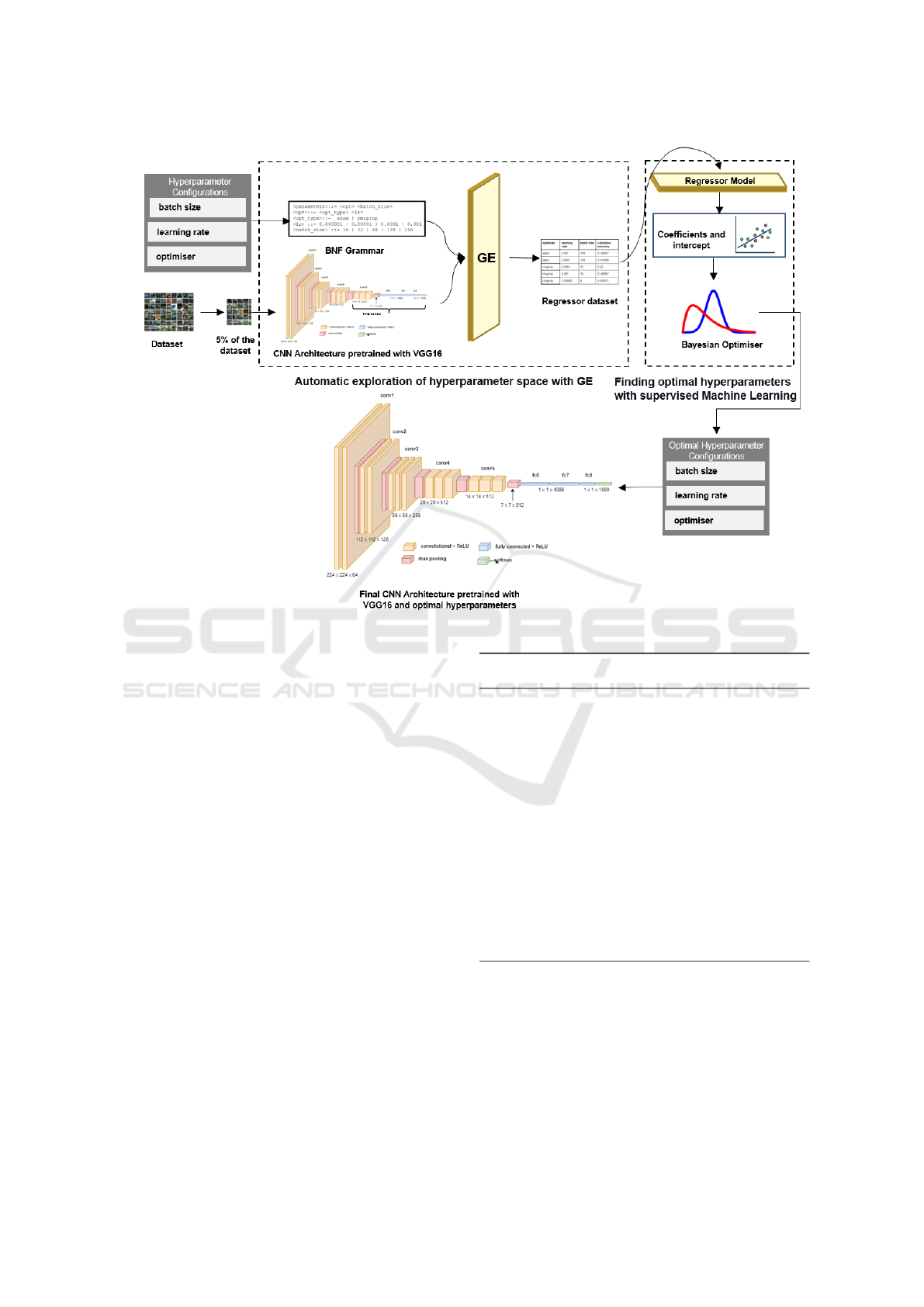
Figure 1: Pipeline of the HyperEstimator Model.

GE (Ryan, 2010; O’Neill and Ryan, 2001; Ryan et al.,

2018) is an evolutionary algorithm that evolves a so-

lution from the search space for a given problem with

the evolutionary strategies. The key functionality of

genotype to phenotype mapping with Backus-Naur

Form (BNF) (Ryan, 2010) grammar in GE generates

syntactically correct phenotypes, and makes it pro-

gramming language independent and hence, useful

across multiple problem domains. In the proposed

system, the search space of hyperparameter conﬁg-

uration of the CNN model is converted to BNF gram-

mar. The CNN architecture is then evolved using 5%

of the training dataset. The phenotypes of the popula-

tion in the search space of GE and their ﬁtness scores

(Lima et al., 1996) are collected for the last genera-

tion, in our case, the 5

generation, in a separate ﬁle

to feed to the regressor model.

3.2 Finding Optimal Hyperparameters

with Supervised Machine Learning

A linear regressor model is a ML technique that ex-

tracts the relationship between one or more explana-

tory variable and the target variable (Bindra et al.,

2021). The dependent variables are hyperparameters

, H

. . . , H

} and the predictor variable is the

Algorithm 1: Automatic exploration of hyperparameter

space with Grammatical Evolution.

Input: BNF Grammar, CNN architecture, 5% of the

image dataset, generation size gen size, popula-

tion size pop size

Output: Dataset of phenotypes of the individuals

and their ﬁtness

1: for g = 1 to gen size do

2: for p = 1 to pop size do

3: I

= Phenotype of the individual

from the BNF Grammar

4: V

= Fitness of the individual I

5: end for

6: if g is equal to the last generation then

Add I

and V

to the individuals.csv ﬁle

7: end if

8: end for

validation accuracy. The regressor model performs

the feature extraction and predicts the weights for

each of the hyperparameter conﬁgurations and the in-

tercept, by minimising the regression loss as deﬁned

in Algorithm 2.

The Bayesian Optimiser (Bindra et al., 2021),

which is based on the maximum likelihood function,

then uses this regression model to predict the optimal

ICSBT 2022 - 19th International Conference on Smart Business Technologies

Algorithm 2: Finding optimal hyperparameters with super-

vised Machine Learning - Regressor Model.

Input: Individuals from individuals.csv ﬁle returned

by GE

Output: Weights {w

, w

, ...w

} and intercept α

1: while w

not converged do

2: Initialise the weights {w

, w

, ...w

} and

intercept α with random values

3: validation accuracy

predicted

= α + H

+ ... + H

4: error =

∑

instances

i=1

(validation accuracy

actual

−

validation accuracy

predicted

)

5: Update weights {w

, w

, ...w

} and intercept

α to minimize error

6: end while

hyperparameters for the CNN model as deﬁned in Al-

gorithm 3. The Bayesian Optimiser maximises the

validation accuracy (objective function). The CNN

model is then trained on the entire dataset with the

optimal hyperparameters obtained from the HyperEs-

timator.

Algorithm 3: Finding optimal hyperparameters with super-

vised Machine Learning - Bayesian Estimator.

Input: Hyperparameter space D, number of

iterations n, target objective function

validation accuracy = α + H

+ H

... + H

Output: Optimal hyperparameter conﬁguration

HC = {H

, H

. . . , H

}

1: Set initial hyperparameter conﬁguration HC =

, H

. . . , H

}

2: Evaluate the objective function

validation accuracy

3: while i < n do

4: Select new hyperparameter conﬁguration

n+1

by optimizing the acquisition

function a: HC

n+1

= HC a(HC, D)

5: Evaluate the objective function

validation accuracy

n+1

6: Augment

n+1

, (HC

n+1

, validation accuracy

n+1

)}

7: Update model

8: end while

3.3 HyperEstimator Computational

Complexity

The computational complexity of our approach can

be seen as a combination of the complexity of all ML

techniques used in the pipeline. Hence, we can deﬁne

the complexity of the HyperEstimator as in Equation

(3).

O(HyperEstimator) = O(GE) + O(LR) + O(BO)

(3)

where O(GE) is the computational complexity of

the GE model, O(LR) is the computational complex-

ity of the linear regressor and O(BO) is the compu-

tational complexity of the Bayesian Optimizer. The

computational complexity for Bayesian Optimization

is known to be O(x

) (Lan et al., 2022), where x is

the total number of candidate solution evaluations.

The computational complexity for the linear regres-

sion model is O(k

(n + k)), where n is the number of

observation and k is the number of weights (Baner-

jee, 2020). GE is an evolutionary approach driven by

an evolutionary search engine. In this research work,

we have used GE driven by Genetic Algorithms (GA).

Hence, computational complexity for GE is the com-

plexity for GA and GE. The complexity for GA is de-

ﬁned as computational efforts for the evaluation of the

individuals. This leads to an overall complexity of GE

as the product of complexity ﬁtness function and the

number of ﬁtness evaluations.

O(GE) = O( f itness f unction) ∗ (# f itness evaluations)

(4)

The computational efforts of the ﬁtness evalu-

ations are determined by the population size, size

of each individual and number of generations, and

the genetic parameters used such as crossover and

mutation. However, according to (Oliveto and Witt,

2015), as the time for genetic parameters applied

is same for each individual, we do not consider it

in the computational efforts and it is considered

as O(1). Hence, the number of ﬁtness evaluations

can be calculated as #o f f itness evaluations =

(population size)(size o f individual)

(#o f generations). The complexity of the ﬁtness

function in our case is the complexity of the

CNN architecture. To determine it, the number

of ﬂoating-point operations (FLOPs) (Molchanov

et al., 2016) are assessed for each layer in the CNN

model. Combining all these individual computational

complexities, we get the overall complexity of our

approach. Hence, the computational complexity is as

deﬁned in Equation (5).

O(HyperEstimator) = O(GE)+O(x

)+O(k

(n+k))

(5)

HyperEstimator: Evolving Computationally Efﬁcient CNN Models with Grammatical Evolution

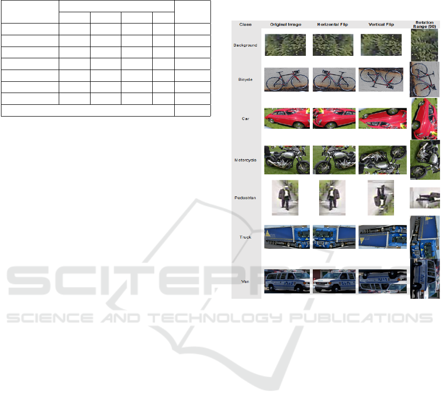
Table 1: Dataset Details. S1: MIO-TCD, S2: TAU Vehicle,

S3: DelftBikes, S4: PASCAL VOC 2012.

Class

Data Source

Total

S1 S2 S3 S4

bicycle 2284 1618 1098 - 5000

car 3000 2000 - - 5000

motorcycle 1982 2986 - 32 5000

pedestrian 5000 - - - 5000

van 4000 1000 - - 5000

background 5000 - - - 5000

truck 3000 2000 - - 5000

Total 35000

4 EXPERIMENTAL SETUP

This section discusses the dataset details and experi-

mental setup for our approach.

4.1 Dataset Details

The dataset we used in our experiments are a combi-

nation of several sources which include labelled ve-

hicle images. We combined them and created a sub-

set consisting only of different vehicle classes. The

datasets involved in this process are:

• The MIOvision Trafﬁc Camera Dataset (MIO-

TCD) dataset, which was released as a part of

challenge in CVPR 2017 (Luo et al., 2018)

• TAU Vehicle Type Recognition Competition

dataset from Kaggle (tau, 2020)

• DelftBikes (Kayhan et al., 2021)

• PASCAL VOC 2012 dataset (Everingham et al., )

The MIO-TCD contains 11 different classes of ve-

hicles for image classiﬁcation and object detection

tasks while TAU Vehicle data contains 36,500 images

for 17 different classes of vehicle. DelftBikes con-

tains 10,000 bike images while PASCAL VOC con-

tains 20 object categories. There was a couple of mo-

tivation behind combining these four datasets:

• To have a balanced dataset for each vehicle class

and hence avoid the problem of bias.

• To have a sufﬁciently large dataset for training the

CNN model to avoid problems related to overﬁt-

ting.

In the real-time video captured in some Indian

cities, we observe the following classes of vehicles:

{background, bicycles, car, trucks, van, motorcycle,

pedestrian}. As the objective of the experiments was

to test the CNN model on the above real-time trafﬁc

videos, we selected only those classes as mentioned

above from the MIO-TCD dataset. We have used 7

classes for training with 5000 images in each class.

The distribution of images from each of the datasets

into respective classes is shown in Table 1.

Figure 2: Sample images for each class from the image

dataset with data augmentation techniques.

4.2 CNN Architecture

For the experiments, we used the VGG-16 model and

incorporated transfer learning by using the pretrained

weights from the Imagenet (Deng et al., 2009) dataset.

The CNN architecture used was the same as that of the

literature (Kshirsagar et al., 2022; Kshirsagar et al.,

2021). Hence, we used the same CNN architecture for

a fair comparison. We followed the process of freez-

ing 70% of the layers while training only the remain-

ing 30% of layers. The activation function used for

the last layer was Softmax with 7 neurons, each rep-

resenting a vehicle class and the image size, 224x224.

The dataset was distributed into 80% for training and

20% for testing purposes. We augmented the image

data by horizontal ﬂip, vertical ﬂip and rotating the

images by 90

◦

for robust training of the model. Fig-

ure 2 illustrates the samples of augmented images for

each class of the dataset. The steps per epoch were

calculated by dividing the number of training samples

by the batch size while the validation steps were cal-

culated by dividing the test samples by the batch size.

ICSBT 2022 - 19th International Conference on Smart Business Technologies

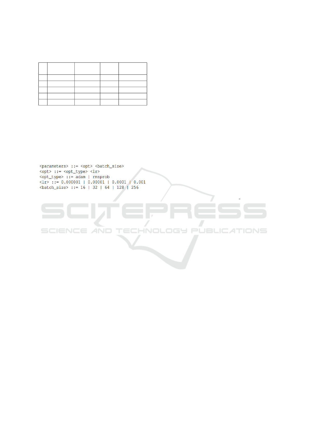
Table 2: Sample individuals obtained during evolutionary

runs.

# optimiser

learning

rate

batch

size

validation

accuracy

1 adam 0.001 128 0.142857

2 adam 0.0001 128 0.574286

3 rmsprop 0.0001 32 0.52

4 rmsprop 0.001 16 0.142857

5 rmsprop 0.000001 8 0.428571

5 RESULTS

The hyperparameter space for the model consisted of

{learning rate, batch size and optimiser}. The hyper-

parameter space was transformed into BNF grammar

as shown in Figure 3 and fed to the GE model (Bal-

dominos et al., 2018; de Lima et al., 2019).

Figure 3: BNF Grammar deﬁning the hyperparameters of

the CNN model.

A ﬁtness function evaluates how well the indi-

viduals are performing in an evolutionary algorithm.

In this research work, the evolved CNN models

were evaluated by deﬁning validation accuracy of the

model as the ﬁtness function with the goal of max-

imising it. The choice of values for each of the hyper-

parameters forms an individual or chromosome. e.g.,

one of the sample chromosomes from the BNF gram-

mar can be adam 0.0001 128. Using the CNN archi-

tecture and 5% of the data from our dataset, we per-

formed evolutionary runs with the BNF grammar for

5 epochs where the parameter setup was as follows:

population size: 10, generations: 5, tournament size:

2, elitism, initialization: sensible. The experiments

were performed using PonyGE2 (Fenton et al., 2017),

the Python tool for GE using TensorFlow and keras

library, and trained on Quadro RTX 8000 - Nvidia

GPU. We stored all the candidate individuals from the

generation in a .csv ﬁle to be used for the next step

in our proposed pipeline. Sample values of the indi-

viduals generated during the evolutionary process are

shown in Table 2.

The .csv ﬁle of the candidate solutions for the hy-

perparameter space was then ﬁtted to a linear regres-

sion model to ﬁnd the values of coefﬁcients for the

equation (6).

F = H

+ H

+ α (6)

validation accuracy was the dependent variable

while the independent variables were {optimiser,

learning rate, batch size}. The Python library

statsmodels (Seabold and Perktold, 2010) was

used to ﬁt the data into linear regression model.

The values for {w

, w

} and α obtained were

as follows: −3.18194782e − 02, −3.80413117e +

02, −3.09998001e −04 and 0.6085946681414556 re-

spectively. Replacing the values for the coefﬁcients

we get the following regression model as seen in

equation (7).

F = (−3.18194782e

−02

) + (−3.80413117e

+02

)

+(−3.09998001e

−04

0.6085946681414556

(7)

Maximum likelihood function was then used to get

the best value of the hyperparameters for the CNN

model with Bayesian Optimiser. The hyperopt

(Bergstra et al., 2013) library was used to estimate

the optimal values of hyperparameters. The hyper-

opt library contains a f

min

function that minimizes the

target. In our case, the target function was validation

accuracy with an objective to maximise it, hence f

min

was the reciprocal of validation accuracy. hyperopt

contains a parameter, named as max evals, that de-

ﬁnes the number of conﬁgurations that the Bayesian

Optimiser tries. This parameters is useful while track-

ing the subspaces of hyperparameters and their ex-

plainability. The following were found to be the

best with Bayesian Optimiser: {H

(optimizer): adam,

(learning rate): 0.000001, H

(batch size): 16 }.

The optimal hyperparameters obtained from our

approach HyperEstimator were then used to train the

CNN model on the entire dataset over 40 epochs, with

an early stopping for the ﬁnal model. The dataset was

divided into 80% for training and 20% for validation.

It took around 6 hours to train the CNN model with

the optimal hyperparameters, achieving a validation

accuracy score of 87%.

5.1 Comparative Analysis

In order to compare the results to those obtained in

the literature, we also ran an experiment without the

HyperEstimator approach using the hyperparameters

as used in the literature (Kshirsagar et al., 2022).

The CNN architecture was the same in both the ap-

proaches, only differing in the hyperparameters.

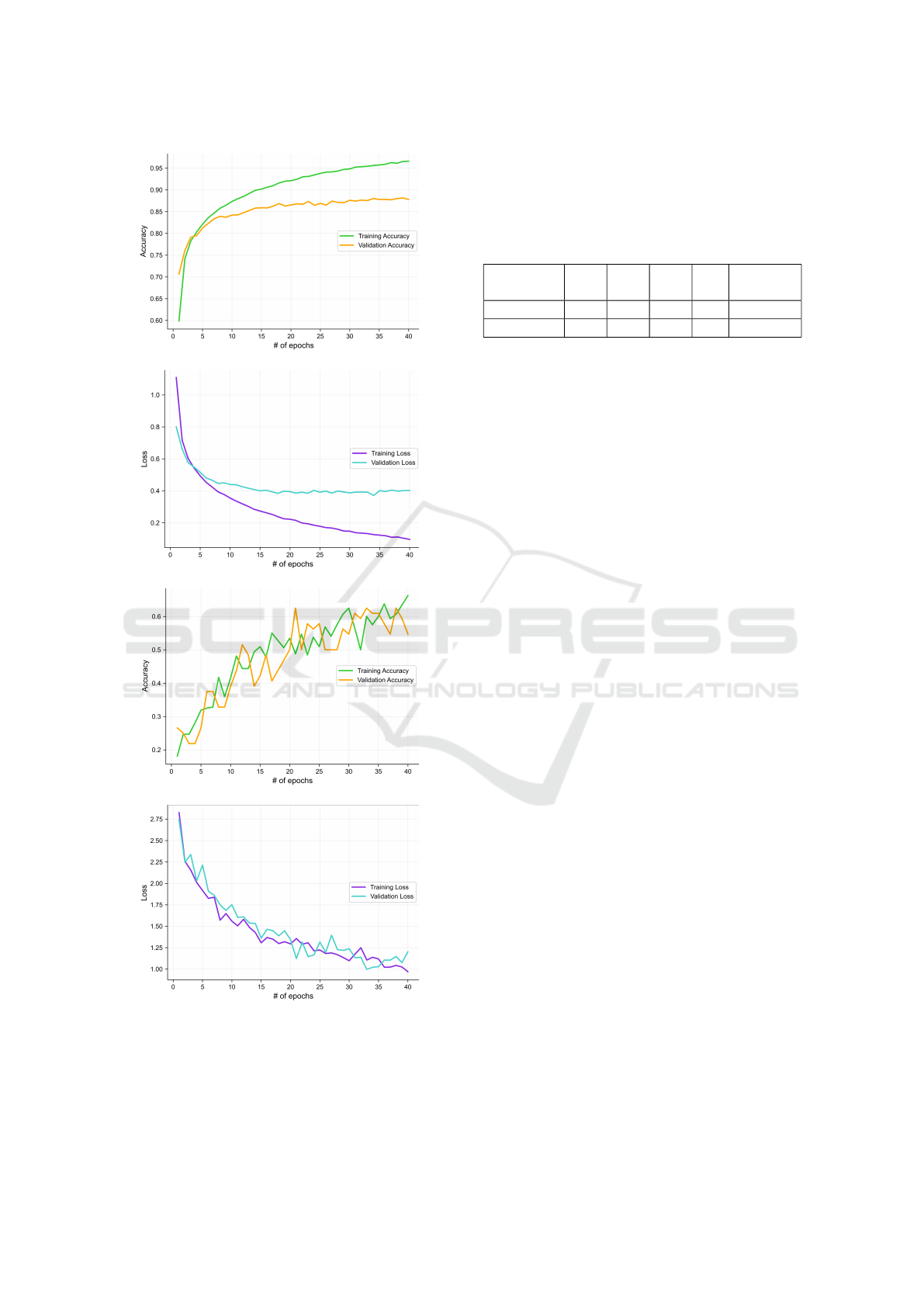
The performance of training and validation ac-

curacies and losses across the epochs for both ap-

proaches are as illustrated in Figure 4. It can be ob-

served from the graphs that there is a dramatic im-

provement in the validation accuracy when the model

was trained with the hyperparameters tuned with Hy-

HyperEstimator: Evolving Computationally Efﬁcient CNN Models with Grammatical Evolution

(a)

(b)

(c)

(d)

Figure 4: (a) Training and Validation accuracy and (b)

Training and Validation loss for CNN models trained with

hyperparameters with HyperEstimator (c) Training and Val-

idation accuracy and (d) Training and Validation loss for

CNN model trained with hyperparameters from (Kshirsagar

et al., 2022).

Table 3: Qualitative analysis between models pre- and post-

tuning with HyperEstimator. The pre-training model is re-

ferred from the literature (Kshirsagar et al., 2022). TA:

Training Accuracy, TL: Training Loss, VA: Validation Ac-

curacy, VL: Validation Loss. #1 Hyperparameters tuned

without HyperEstimator, #2 Hyperparameters tuned with

HyperEstimator.

Approach TA TL VA VL

Time

(mins)

#1 0.66 0.9 0.54 1.2 3 mins

#2 0.96 0.09 0.87 0.4 365 mins

perEstimator as compared to the model without using

HyperEstimator. The validation accuracies for both

the approaches are illustrated in Figure 4a and Fig-

ure 4c respectively. The validation accuracy achieved

with the model tuned with HyperEstimator was 87%

while that with without HyperEstimator was only

54%. We also observe a signiﬁcant improvement

in validation loss when the model was trained with

the hyperparameters tuned with HyperEstimator, as

shown in Figure 4b and Figure 4d. The comparative

analysis of both the approaches in terms of accuracy

and loss at 40

epoch is presented in Table 3. As can

be observed in column 4, the model’s validation accu-

racy has improved signiﬁcantly, though the time taken

for the model training was competitively high.

We also plotted the confusion matrix against the test

data to understand how well the model performed for

each class. Figure 5 shows the confusion matrix for

both the approaches on the test dataset. All the classes

were balanced and the accuracy has been normalized

while plotting the confusion matrix; hence, each row

will sum up to 1. In the plots, we can observe the

CNN model tuned with HyperEstimator has learnt

the major parameters for each class as compared to

the traditional approach as illustrated in Figure 5a and

Figure 5b. The model has achieved the maximum ac-

curacy in classifying the background class with an ac-

curacy of 96%. On the other hand, the model seems to

misclassify the bicycle as motorcycle and pedestrian

and vice versa. This may be due to the fact that the

structures of motorcycles and bicycles are similar in a

way and the images for pedestrian are blurred. This

indicates the model still has scope to learn the features

for these classes. Similar is the case with the classes,

truck and van; the model misclassiﬁes the truck with

van and vice versa. This may be again due to the over-

lapping of the visual structures.

5.2 Model validation

The CNN model was tested against the real-world

benchmark CIFAR10 (Krizhevsky, 2009) and CI-

FAR100 (Krizhevsky, 2009) datasets. CIFAR10

ICSBT 2022 - 19th International Conference on Smart Business Technologies

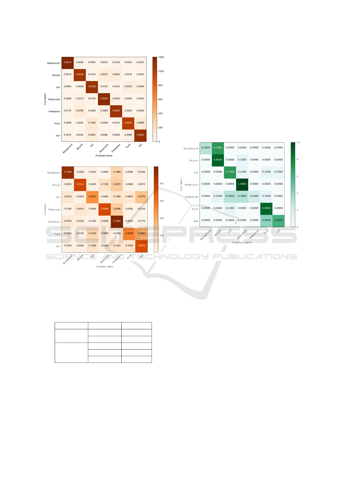
(a)

(b)

Figure 5: Confusion matrix plots for CNN model trained

with 40 epochs and tested on test dataset with (a) Hyperpa-

rameters tuned with HyperEstimator; (b) Hyperparameters

tuned without HyperEstimator.

Table 4: Comparative analysis of the CNN model tuned

with HyperEstimator on real-world benchmark datasets.

Dataset Classes Accuracy

CIFAR10

Car 0.64

Truck 0.57

CIFAR100

Bicycle 0.88

Motorcycle 0.45

Truck 0.71

dataset consists of a total of 60000 images across 10

classes, 5000 images per class for training and 1000

per class for testing. The size of the images is 32x32

in 3 color channels. CIFAR100 dataset consists of

60000 images across 100 classes, with 500 images

per class for training and 100 per class for testing pur-

poses. The images in CIFAR100 are of size 32x32

with 3 color channels. For CIFAR10, we had two

similar classes in our dataset car and truck while for

CIFAR100, we had three similar classes, bicycle, mo-

torcycle and truck. While testing the images were

upscaled to 224x224 as our CNN model had the in-

put size of 224x224 and we tested the performance

of our proposed model on these classes for CIFAR10

and CIFAR100 datasets. Table 4 shows the accuracy

for each of the class against the CNN model evolved

with HyperEstimator. From the tables we can infer

that the model has good accuracy against real-world

benchmark datasets.

Figure 6: Confusion matrix plot for the CNN model

tuned with HyperEstimator against real-world trafﬁc video

dataset.

5.3 Model Testing

To test the performance of the CNN model, we cap-

tured the real-time videos of the trafﬁc in some Indian

cities. We collected three videos of one minute each

during daytime and at night. We divided the videos

into frames and predicted the class obtained with the

CNN model. We used 70 frames in total, 10 images

per class for testing. The accuracy obtained was 0.65.

Figure 7 illustrates the confusion matrix plot for the

testing of the video dataset for each class. The re-

sults imply that the model tuned with HyperEstimator

performs well in real-world scenarios for most of the

class while there is still some scope for improvement

against background and pedestrian class.

5.4 Interpretability of HyperEstimator

While using the trained AI models in real-world

scenarios, it is critical to understand which param-

eters are important and how the model has learnt

HyperEstimator: Evolving Computationally Efﬁcient CNN Models with Grammatical Evolution

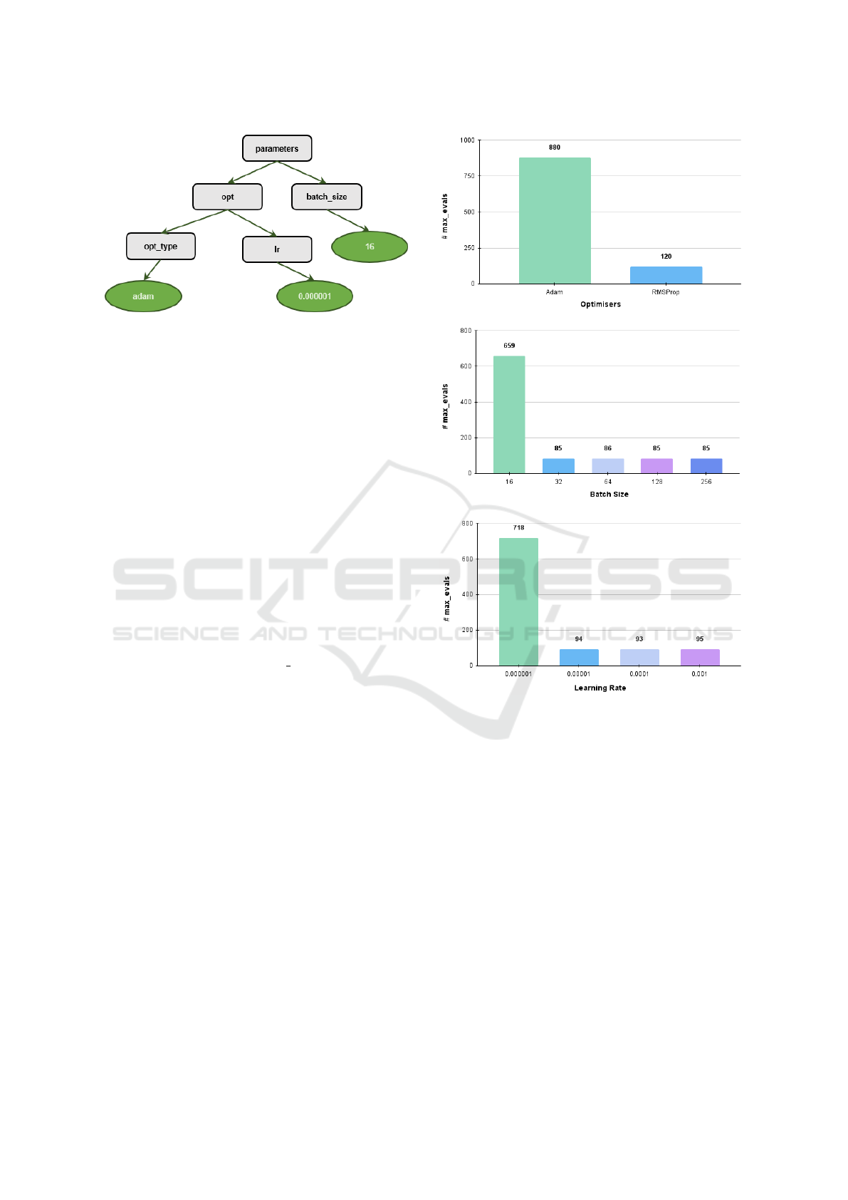
Figure 7: Example derivation tree from BNF grammar.

them for their trustworthiness. Explainable AI (XAI)

(Holzinger, 2018) motivates the research for such

models to explain their decisions. In this research

work, HyperEstimator uses three key ML techniques

all of which can be explainable for their results. GE

uses genotype to phenotype mapping and generates

a derivation tree for the individuals. This helps in

understanding the solutions in human understandable

form. The derivation tree in Figure 7 is obtained from

BNF grammar, as shown in Figure 3. The statsmodels

library from Python used for linear regression is inter-

pretable. It displays all the metadata (statistical tests,

conﬁdence intervals, etc.) about the regression model

in human understandable form. Similarly, Bayesian

Optimiser is a probabilistic way of optimizing and

incorporating explainability into the HyperEstimator

system. In this research work, we have visualized

the values of the features contributing to the target

function in Bayesian Optimiser with hyperopt library.

As explained in Section 5, max evals determines the

number of trials that the model uses to ﬁnd the opti-

mal hyperparameters. These trials can be visualised

to analyse the contributions of each sub-space of the

hyperparameters across the trials. Figure 8 illustrates

the sub-spaces of hyperparameters in Bayesian Opti-

miser model. The ﬁgures clearly illustrate the major

contributions of the optimal values across the trials.

In this way, all the ML techniques of HyperEstimator

system illustrate interpretability.

6 CONCLUSIONS AND FUTURE

SCOPE

In this research work, we propose HyperEstimator,

a system consisting of a suite of ML techniques to

reduce the computational efforts for tuning hyperpa-

rameters of CNN models. We employed GE for the

hyperparameter search space whereas the Bayesian

Optimiser exploited the local search space for the op-

timal values of hyperparameters. We present a case

Figure 8: Feature subsets with their contribution in estimat-

ing optimal hyperparameters for Bayesian Optimiser.

study on a real-world trafﬁc image dataset and pro-

pose to use only 5% of the training data for hyper-

parameter tuning, to reduce the computational cost.

With the obtained conﬁgurations for hyperparame-

ters, we could signiﬁcantly improve the validation ac-

curacy to 87% for the CNN model. Initial results from

our approach tested against the real-world benchmark

datasets, CIFAR10 with two overlapping classes, viz.

car and trucks, and CIFAR100 with three overlapping

classes, viz. bicycle, motorcycle and truck, suggested

the strong potential about our approach. The evolved

CNN model was also tested against real-world traf-

ﬁc video datasets as a case study which resulted into

65% accuracy from a sample of 70 frames from the

videos. The use of GE and Bayesian Optimiser also

leads to explainability of the proposed approach. The

ICSBT 2022 - 19th International Conference on Smart Business Technologies

immediate future scope to this approach is to extend

the hyperparameters we consider to tune.

ACKOWLEDGEMENTS

This work was supported by the Science Foundation

Ireland Grant #16/IA/4605.

REFERENCES

(2020). Tau vehicle type recognition competition.

Ahmadizar, F., Soltanian, K., AkhlaghianTab, F., and Tsou-

los, I. (2015). Artiﬁcial neural network development

by means of a novel combination of grammatical evo-

lution and genetic algorithm. Engineering Applica-

tions of Artiﬁcial Intelligence, 39:1–13.

Andonie, R. and Florea, A. (2020). Weighted random

search for CNN hyperparameter optimization. CoRR,

abs/2003.13300.

Assunc¸

ao, F., Lourenc¸o, N., Machado, P., and Ribeiro, B.

(2018). Evolving the Topology of Large Scale Deep

Neural Networks, pages 19–34.

Baldominos, A., Saez, Y., and Isasi, P. (2018). Evolution-

ary design of convolutional neural networks for hu-

man activity recognition in sensor-rich environments.

Sensors, 18(4).

Banerjee, W. (2020). Train/Test Complexity and Space

Complexity of Linear Regression.

Bergstra, J., Yamins, D., and Cox, D. (2013). Making a

science of model search: Hyperparameter optimiza-

tion in hundreds of dimensions for vision architec-

tures. In Dasgupta, S. and McAllester, D., editors,

Proceedings of the 30th International Conference on

Machine Learning, volume 28 of Proceedings of Ma-

chine Learning Research, pages 115–123, Atlanta,

Georgia, USA. PMLR.

Bindra, P., Kshirsagar, M., Ryan, C., Vaidya, G., Gupt,

K. K., and Kshirsagar, V. (2021). Insights into the

advancements of artiﬁcial intelligence and machine

learning, the present state of art, and future prospects:

Seven decades of digital revolution. In Satapathy,

S. C., Bhateja, V., Favorskaya, M. N., and Adilakshmi,

T., editors, Smart Computing Techniques and Applica-

tions, pages 609–621, Singapore. Springer Singapore.

Bochinski, E., Senst, T., and Sikora, T. (2017). ‘Hyper-

parameter optimization for convolutional neural net-

work committees based on evolutionary algorithms‘,

2017 IEEE International Conference on Image Pro-

cessing (ICIP), Beijing, China, Sept. 17-20, 2017,

3924-3928, available: http://dx.doi.org/10.1109/ICIP.

2017.8297018.

de Lima, R. H. R., Pozo, A. T. R., and Santana, R. (2019).

Automatic design of convolutional neural networks

using grammatical evolution. 2019 8th Brazilian Con-

ference on Intelligent Systems (BRACIS), pages 329–

334.

Deng, J., Dong, W., Socher, R., Li, L.-J., Li, K., and Fei-

Fei, L. (2009). Imagenet: A large-scale hierarchical

image database. In 2009 IEEE Conference on Com-

puter Vision and Pattern Recognition, pages 248–255.

Everingham, M., Van Gool, L., Williams, C. K. I., Winn,

J., and Zisserman, A. The PASCAL Visual Object

Classes Challenge 2012 (VOC2012) Results.

Fenton, M., McDermott, J., Fagan, D., Forstenlechner, S.,

Hemberg, E., and O’Neill, M. (2017). Ponyge2:

Grammatical evolution in python. In Proceedings of

the Genetic and Evolutionary Computation Confer-

ence Companion, GECCO ’17, page 1194–1201, New

York, NY, USA. Association for Computing Machin-

ery.

Ghosh, A., Suﬁan, A., Sultana, F., Chakrabarti, A., and De,

D. (2020). Fundamental Concepts of Convolutional

Neural Network, pages 519–567. Springer Interna-

tional Publishing, Cham.

He, K., Zhang, X., Ren, S., and Sun, J. (2015). Deep

residual learning for image recognition. CoRR,

abs/1512.03385.

Holzinger, A. (2018). From machine learning to explainable

ai. In 2018 World Symposium on Digital Intelligence

for Systems and Machines (DISA), pages 55–66.

Kayhan, O., Vredebrecht, B., and van Gemert, J. (2021).

DelftBikes, data underlying the publication: Hallu-

cination In Object Detection-A Study In Visual Part

Veriﬁcation.

Krizhevsky, A. (2009). Learning multiple layers of features

from tiny images. Technical report.

Kshirsagar, M., Lahoti, R., More, T., and Ryan, C. (2021).

Greecope: Green computing with piezoelectric effect.

pages 164–171.

Kshirsagar, M., More, T., Lahoti, R., Adgaonkar, S., Jain,

S., and Ryan, C. (2022). Rethinking trafﬁc manage-

ment with congestion pricing and vehicular routing for

sustainable and clean transport. In Proceedings of the

14th International Conference on Agents and Artiﬁ-

cial Intelligence - Volume 3: ICAART,, pages 420–

427. INSTICC, SciTePress.

Lan, G., Tomczak, J. M., Roijers, D. M., and Eiben,

A. (2022). Time efﬁciency in optimization with a

bayesian-evolutionary algorithm. Swarm and Evolu-

tionary Computation, 69:100970.

Lecun, Y., Bottou, L., Bengio, Y., and Haffner, P. (1998).

Gradient-based learning applied to document recogni-

tion. Proceedings of the IEEE, 86(11):2278–2324.

Lima, J., Gracias, N., Pereira, H., and Rosa, A. (1996).

Fitness function design for genetic algorithms in cost

evaluation based problems. In Proceedings of IEEE

International Conference on Evolutionary Computa-

tion, pages 207–212.

Luo, Z., Branchaud-Charron, F., Lemaire, C., Konrad, J.,

Li, S., Mishra, A., Achkar, A., Eichel, J., and Jodoin,

P.-M. (2018). Mio-tcd: A new benchmark dataset for

vehicle classiﬁcation and localization. IEEE Transac-

tions on Image Processing, 27(10):5129–5141.

Miikkulainen, R., Liang, J., Meyerson, E., Rawal, A., Fink,

D., Francon, O., Raju, B., Shahrzad, H., Navruzyan,

HyperEstimator: Evolving Computationally Efﬁcient CNN Models with Grammatical Evolution

A., Duffy, N., and Hodjat, B. (2017). Evolving deep

neural networks.

Molchanov, P., Tyree, S., Karras, T., Aila, T., and Kautz,

J. (2016). Pruning convolutional neural networks for

resource efﬁcient inference.

Ng, A. (2021a). Andrew ng: Don’t buy the ’big data’ a.i.

hype — fortune.

Ng, A. (2021b). Data-centric ai competition.

Ng, A. (2022). Andrew ng: Unbiggen ai - ieee spectrum.

Oliveto, P. S. and Witt, C. (2015). Improved time complex-

ity analysis of the simple genetic algorithm. Theoreti-

cal Computer Science, 605:21–41.

O’Neill, M. and Ryan, C. (2001). Grammatical evolu-

tion. IEEE Transactions on Evolutionary Computa-

tion, 5(4):349–358.

Ryan, C. (2010). Grammatical evolution tutorial. In Pro-

ceedings of the 12th Annual Conference Companion

on Genetic and Evolutionary Computation, GECCO

’10, page 2385–2412, New York, NY, USA. Associa-

tion for Computing Machinery.

Ryan, C., O’Neill, M., and Collins, J. (2018). Handbook of

Grammatical Evolution.

Seabold, S. and Perktold, J. (2010). statsmodels: Econo-

metric and statistical modeling with python. In 9th

Python in Science Conference.

Simonyan, K. and Zisserman, A. (2014). Very deep convo-

lutional networks for large-scale image recognition.

Stanley, K. O. and Miikkulainen, R. (2002). Evolving neu-

ral networks through augmenting topologies. Evolu-

tionary Computation, 10(2):99–127.

Szegedy, C., Liu, W., Jia, Y., Sermanet, P., Reed, S.,

Anguelov, D., Erhan, D., Vanhoucke, V., and Rabi-

novich, A. (2014). Going deeper with convolutions.

Tsoulos, I., Gavrilis, D., and Glavas, E. (2008). Neu-

ral network construction and training using grammat-

ical evolution. Neurocomputing, 72(1):269–277. Ma-

chine Learning for Signal Processing (MLSP 2006) /

Life System Modelling, Simulation, and Bio-inspired

Computing (LSMS 2007).

Yu, T. and Zhu, H. (2020). Hyper-parameter optimiza-

tion: A review of algorithms and applications. CoRR,

abs/2003.05689.

APPENDIX

The datasets used in the experiments and the

code for HyperEstimator can be found at

https://github.com/gauriivaidya/HyperEstimator.

ICSBT 2022 - 19th International Conference on Smart Business Technologies