Contribution to Robot System Identification: Noise Reduction using a
State Observer
Bilal Tout
1
, Jason Chevrie
1
, Laurent Vermeiren
1
and Antoine Dequidt
1,2
1
Univ. Polytechnique Hauts-de-France, LAMIH, CNRS, UMR 8201, F-59313 Valenciennes, France
2
INSA Hauts-de-France, F-59313 Valenciennes, France
Keywords:
System Identification, Robot Dynamics, Kalman Filter, Least Squares Estimation.
Abstract:
Conventional identification approach based on the inverse dynamic identification model using least-squares
and direct and inverse dynamic identification techniques has been effectively used to identify inertial and
friction parameters of robots. However these methods require a well-tuned filtering of the observation matrix
and the measured torque to avoid bias in identification results. Meanwhile, the cutoff frequency of the low-
pass filter f
c
must be well chosen, which is not always easy to do. In this paper, we propose to use a Kalman
filter to reduce the noise of the observation matrix and the output torque signal of the PID controller.
1 INTRODUCTION
Robotics applications employing model-based con-
trollers require knowing the system parameters with
high accuracy, particularly in the industrial area as
stated in (Han et al., 2020) and when using impedance
control techniques as described in (Akdo
˘
gan et al.,
2018). In the context of rigid robotics, the conven-
tional identification approach based on the inverse dy-
namic identification model (IDIM) and least-squares
(LS) technique has been effectively used to identify
inertial and friction parameters of many robots.
However, using sensors with large quantization
steps may result in an ill-conditioned observation
matrix constructed from the quantized position and
its derivatives. Furthermore, the amplification of
the quantization error in the integral step of the
PID controller, which is commonly used to control
robotic systems, results in noisy torque measure-
ments. Because of measurement noise and incorrect
data-filtering, LS parameter estimates may become
extremely biased, to the point of losing all physi-
cal consistency, which can be seen in negative link
masses and friction coefficients for example.
(Gautier, 1997) demonstrated that if a well-tuned
filtering of the observation matrix and the measured
torque is employed with LS, good identification re-
sults can be obtained. Other methods robust to noisy
observation matrix were proposed such as direct and
inverse dynamic identification method (DIDIM) in
(Gautier et al., 2013), however they still require some
low-pass filtering of the measured torque signal. In
practice, the cutoff frequency f
c
of the low-pass filter
must be well chosen. (Gautier, 1997) and (Pham et al.,
2001) used the dynamic frequency w
dyn
of the robot
to determine f
c
. Nonetheless w
dyn
is not necessarily
an accessible value and is not always well defined for
non-linear systems. Further, (Swevers et al., 1997)
and (Olsen et al., 2002) demonstrated that Maximum
Likelihood identification method can significantly re-
duce the bias on parameter estimates in the case of
noisy joint measurements, but at the cost of a greater
computational effort.
In this paper, to limit the influence of quantiza-
tion on the observation matrix, we consider integrat-
ing a nonlinear observer and calculating the observa-
tion matrix using the estimated position and velocity
rather than the quantized position and its derivatives.
Then, we propose using the estimated position and ve-
locity as an input to the PID controller to reduce noise
in the measured torque signal.
This paper is organized as follows: background
and existing identification methods for robotic sys-
tems are presented in section 2. Section 3 details the
proposed non-linear Kalman filtering and the usage of
estimated position and velocity to improve the iden-
tification results. Then, section 4 presents simulation
results for the validation of the method and discus-
sions. Finally section 5 includes the conclusion and
future works.
Tout, B., Chevrie, J., Vermeiren, L. and Dequidt, A.
Contribution to Robot System Identification: Noise Reduction using a State Observer.
DOI: 10.5220/0011322600003271
In Proceedings of the 19th International Conference on Informatics in Control, Automation and Robotics (ICINCO 2022), pages 695-702
ISBN: 978-989-758-585-2; ISSN: 2184-2809
Copyright
c
 2022 by SCITEPRESS – Science and Technology Publications, Lda. All rights reserved
695

2 BACKGROUND
2.1 Inverse Dynamic Model
The inverse dynamic model (IDM) of a rigid robot
with n degrees of freedom (DOF) calculates the joint
forces and torques τ ∈ R
n
as a function of joint po-
sitions, velocities and accelerations q, ˙q, ¨q ∈ R
n
. The
IDM can be obtained from the Newton-Euler or the
Lagrangian equations (Khalil and Dombre, 2002) as
follows:
τ = M(q) · ¨q +C(q, ˙q) · ˙q + g(q)+ f ( ˙q), (1)
where M(q) ∈ R
n×n
is the robot inertia matrix,
C(q, ˙q) ∈ R
n×n
is the Coriolis and centrifugal ma-
trix, g(q) ∈ R
n
is the gravitational torque vector, and
f ∈ R
n
is the friction. Several friction models exist
(Bogdan, 2010), a classical one is given by the fol-
lowing:
f
j
= F
v
j
· ˙q
j
+ F
c
j
· sign( ˙q
j
), (2)
with F
v
j
and F
c
j
the viscous and Coulomb’s friction
coefficients of the jth joint respectively.
2.2 Model Reduction
Because the friction model in (2) is a linear function
of parameters, the IDM in (1) can be expressed as
a linear function of the standard dynamic parameters
χ =

χ
T
1
χ
T
2
··· χ
T
n

T
∈ R
p
as follows:
τ = IDM
χ
(q, ˙q, ¨q)χ, (3)
where IDM
χ

¨q, ˙q,q

∈ R
n×p
is
the model regressor and χ
j
=

XX
j
XY
j
XZ
j
YY
j
Y Z
j
ZZ
j
MX
j
MY
j
MZ
j
M
j
I
a
j
F
v
j
F
c
j

T
, j = 1, 2,··· ,n, is the jth link stan-
dard dynamic parameters vector containing:

XX
j
, XY
j
, XZ
j
, YY
j
, Y Z
j
, ZZ
j

the elements
of the inertia tensor;

MX
j
, MY
j
, MZ
j

the elements
of the first moment; M
j
the link mass; I
a
j
the inertia
of the actuator and transmission system; and F
v
j
, F
c
j
the friction parameters.
The robot standard parameters specified in vec-
tor χ can be separated into three groups, as indicated
in (Atkeson et al., 1986): identifiable, unidentifiable,
and identifiable in linear combinations. The base in-
ertial parameters β ∈ R
b
, also known as identifiable
parameters, are the minimum set of inertial param-
eters required to construct a robot’s dynamic model
(Mayeda et al., 1990). (Leboutet et al., 2021) em-
ployed QR decomposition to determine β from the set
of standard parameters χ and referenced some other
ways to do so.
After determining the set of base inertial parame-
ters β, the IDM in (3) can be reduced to the minimal
inverse dynamic model given by
τ = IDM
β
(q, ˙q, ¨q)β, (4)
where IDM
β
(q, ˙q, ¨q) ∈ R
n×b
is the reduced model re-
gressor. In practice, due to measurement errors and
modeling uncertainties, the measured torque τ
m
can
be represented as follows:
τ
m
= IDM
β
(q, ˙q, ¨q)β + e, (5)
where e ∈ R
n
is the error.
During an experiment, the robot is controlled to
follow exciting trajectories that are optimized so that
the observation matrix W is well-conditioned, as de-
scribed by the Fourier series in (Swevers et al., 1997),
and the IDM is sampled with a sampling time T
s
. An
over-determined linear system with r = n · N equa-
tions and b unknowns is obtained for N collected sam-
ples, such that
Y = W (q, ˙q, ¨q)β + ε, (6)
where Y ∈ R
r
is the sampled vector of τ
m
; W (q, ˙q, ¨q) ∈
R
r×b
is the sampled matrix of IDM
β
(q, ˙q, ¨q), referred
to as the observation matrix; and ε ∈ R
r
is the sampled
vector of errors e.
2.3 Identification Methods
2.3.1 Least Squares
Ordinary least squares (OLS) is a widely used method
to identify robot base inertial parameters β. OLS solu-
tion
ˆ
β consists in minimizing the 2-norm of the error
vector ε as follows:
ˆ
β = min
β
||ε||
2
. (7)
Solving (6) using OLS gives the following parameters
estimate
ˆ
β =

W
T
W

−1
W
T
Y. (8)
Supposing that W is a deterministic matrix and ε
is a homoskedastic zero-mean additive independent
Gaussian noise, its covariance matrix C
εε
is such that:
C
εε
= E

ε · ε
T

= σ
ε
2
I
r
, (9)
where E(·) is the expectation operator and I
r
∈ R
r×r
the identity matrix.
An unbiased estimation of the variance σ
2
ε
of the
error vector ε is
ˆ
σ
2
ε
=






Y −W
ˆ
β






2
r − b
. (10)
ICINCO 2022 - 19th International Conference on Informatics in Control, Automation and Robotics
696

The covariance matrix C
ˆ
β
ˆ
β
∈ R
b×b
of the parameter
estimation error is given by
C
ˆ
β
ˆ
β
= E


ˆ
β − β

ˆ
β − β

T

,
=
ˆ
σ
2
ε

W
T
W

−1
, (11)
where the ith diagonal coefficient of C
ˆ
β
ˆ
β
represents
the variance σ
2
ˆ
β
i
of the ith estimated parameter
ˆ
β
i
such
that
σ
2
ˆ
β
i
= C
ˆ
β
ˆ
β
(i,i). (12)
However, if the error vector ε is heteroskedastic, as
is often the case in robotics since the torque noise
level can be different for each joint, the weighted least
squares (WLS) technique can outperform the OLS in
terms of variance. This may be done by weighting (6)
with a matrix G of the inverse of the standard devia-
tion of the error such that G
T
G = C
−1
εε
.
The WLS solution
ˆ
β
W
and the estimation error co-
variance matrix C
ˆ
β
W
ˆ
β
W
in this case can be expressed
as follows:
ˆ
β
W
=

W
T
C
−1
εε
W

−1
W
T
C
−1
εε
Y, (13)
C
ˆ
β
W
ˆ
β
W
=

W
T
C
−1
εε
W

−1
. (14)
OLS and WLS are non-iterative approaches that
obtain base parameter estimates in a single step using
measured or estimated joint torques and joint posi-
tions as illustrated in Fig. 1.
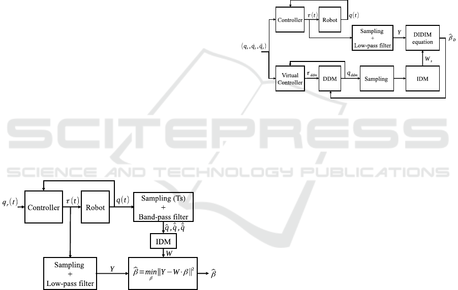
Figure 1: Least squares identification scheme of robot’s
base inertial parameters β considering noisy torque mea-
surements τ and an observation matrix W computed using
the inverse dynamic model (IDM) with quantized position
measurements q and its derivatives of velocity ˙q and accel-
eration ¨q.
However, one issue with the least square (LS)
methods’ parameter estimations is their vulnerability
to measurement noise. Indeed, LS approaches assume
that the observation matrix W and the error vector ε
are uncorrelated, which is not the case in a closed
loop system having measurement noise on the posi-
tion. To overcome this limitation, one option is to
use data filtering (Gautier, 1997), while another is to
employ identification methods that are robust to vio-
lation of this condition such as the one presented in
the following.
2.3.2 Direct and Inverse Dynamic Identification
Method
The direct and inverse dynamic identification method
(DIDIM) proposed by (Gautier et al., 2013) consists
in using simultaneously the inverse dynamic model
and the direct dynamic model (DDM).
As illustrated in Fig. 2, the DIDIM uses only the
measured torque while the observation matrix is con-
structed from the position and its derivatives simu-
lated using the ideal DDM.
Figure 2: Direct and inverse dynamic identification method
(DIDIM) scheme for identification of β considering noisy
torque measurements Y and an observation matrix W
s
com-
puted using the inverse dynamic model (IDM) with position
q
ddm
, velocity ˙q
ddm
and acceleration ¨q
ddm
computed using
the direct dynamic model (DDM) of the robot.
At iteration k, the DIDIM estimate
ˆ
β
k
D
can be iden-
tified using the following equation
ˆ
β
k
D
=

W
k
s
T
W
k
s

−1
W
k
s
T
Y, (15)
where W
k
s
∈ R
r×b
is the observation matrix at itera-
tion k constructed using the noise-free simulated po-
sitions, velocities and accelerations.
It is critical that the system’s trajectory (position,
velocity, and acceleration) do not change significantly
between iterations, such that, for any
ˆ
β
k
D

q
ddm
(
ˆ
β
k
D
), ˙q
ddm
(
ˆ
β
k
D
), ¨q
ddm
(
ˆ
β
k
D
)

≈ (q
r
, ˙q
r
, ¨q
r
).
(16)
In this case, the DIDIM converges in a few iterations
and in some cases in a single iteration as demonstrated
in (Gautier et al., 2013).
After DIDIM convergence, the covariance matrix
of the DIDIM estimate can be calculated through
C
ˆ
β
D
ˆ
β
D
=

W
T
s
C
−1
εε
W
s

−1
. (17)
The benefit of the method is that, measurement
noise filtering is no longer required for the observa-
tion matrix. Nevertheless, noise still exists in the
Contribution to Robot System Identification: Noise Reduction using a State Observer
697

torque measurements, therefore torque filtering is still
required.
2.4 Data Filtering
To produce acceptable identification results in prac-
tice, due to quantification noise in position q and the
noise resulting from the derivative of this position to
calculate the velocity ˙q (see Fig. 4) and accelera-
tion ¨q, filtering the torque and the observation ma-
trix is required when using the LS approach. Without
filtering, estimations may become biased and possi-
bly lose their physical consistency. On the contrary,
the DIDIM technique just needs the measured torque
provided by the the output of the PID controller fre-
quently used in practice. Nonetheless, filtering is still
required to eliminate torque noise (see Fig. 6) caused
by the quantized signals used as the PID controller’s
input.
A simple low-pass filter is often used for filtering
(Gautier, 1997), (Brunot et al., 2018). In both LS and
DIDIM identification approaches, a well-tuned cut-
off frequency f
c
is required. Studies in the literature,
such as (Gautier, 1997) and (Gautier et al., 2013),
use a cut-off frequency f
c
> 10 w
dyn
, where w
dyn
is the system natural frequency, which is not always
known and is not always well defined for non-linear
systems. The nonlinear Coulomb friction may for ex-
ample introduce some high frequency phenomena in
the system. Furthermore, the frequency spectrum of
the noise is often unknown, particularly when consid-
ering quantification noise, thus it is unclear whether
or not this filtering properly removes the noise.
As a result, an alternative processing method is
presented in this paper. It allows estimating better po-
sition and velocity from noisy measures using a non-
linear observer, which is easier to adjust than a low-
pass filter. Furthermore, the observer’s output may be
used as input to the PID controller instead of the quan-
tized signals, allowing the computed torque to be less
noisy.
3 IDENTIFICATION USING A
NONLINEAR OBSERVER
3.1 Extended Kalman Filter
We propose using the extended Kalman filtering
methods, commonly employed for state estimation, to
improve identification results. In this approach, the
state is considered to be x =

q
T
˙q
T

T
∈ R
2·n
. Thus,
the state space model can be obtained using the DDM
computed from the IDM in (1) as:
˙x =

˙q
¨q

=

˙q
DDM
χ
(q, ˙q,τ)

,
=

˙q
M(q)
−1
(τ −C(q, ˙q) ˙q − g(q) − f ( ˙q))

. (18)
The discretization of (18) leads to the state transition
function:
x
k+1
= x
k
+ ˙x
k
(x
k
,τ
k
,w
k
) · T
s
, (19)
where T
s
is the sampling time and we choose to model
the process noise w
k
∼ N (0
b×1
,Q) as a non-additive
noise affecting the dynamic parameters of the system,
with Q ∈ R
b×b
its covariance matrix, such that
Q =





σ
2
w
1
(0)
σ
2
w
2
.
.
.
(0) σ
2
w
b





, (20)
where σ
2
w
i
, i = 1, · ·· , b, is the variance of the error
on the ith parameter
ˆ
β
i
of the estimate vector
ˆ
β. We
introduce a new set of noisy parameters
ˆ
β
i
, that takes
into account the percentage of the uncertainty on the
estimated parameters
ˆ
β
i
as follows:
ˆ
β
i
= (1 + w
i
) ·
ˆ
β
i
(21)
Choosing small values of σ
w
i
indicate high confidence
in the current parameters estimates
ˆ
β. However, large
values indicate that the model is not really trustwor-
thy.
The observation equation also known as the mea-
surement function is given by:
y
k
= q
k
= C · x
k
+ v
k
, (22)
where C = [I
n
0
n
] is a selection matrix and v
k
∼
N (0
n×1
,R) is an additive measurement noise, with
R ∈ R
n×n
its covariance matrix. The benefit of this
formulation is how easily the matrices R and Q may
be adjusted based on physical considerations.
Observer Tuning
To use the extended Kalman filter to estimate position
q and velocity ˙q, the matrices R and Q must be fine-
tuned and the state x and its covariance matrix P well-
initialized. As the robot tracks a reference trajectory
imposed by (q
r
, ˙q
r
, ¨q
r
), the state can initially be set to
x
0
= [q
r
0
˙q
r
0
]
T
and its covariance matrix to P
0
con-
taining values which represent the uncertainty on the
initial values of the position and velocity, small values
indicates high confidence while large values indicates
low confidence.
ICINCO 2022 - 19th International Conference on Informatics in Control, Automation and Robotics
698

Assuming that the quantization error is the major
source of noise in position measurements and under
the assumption that it can be modeled as a white uni-
form noise, its covariance matrix is known to be as
follows (Shardt et al., 2016):
R =





σ
2
v
1
(0)
σ
2
v
2
.
.
.
(0) σ
2
v
n





, with σ
2
v
j
=
(Q
j
quant
)
2
12
,
(23)
where Q
j
quant
, j = 1, ··· , n is the quantization step of
the encoder of the jth joint.
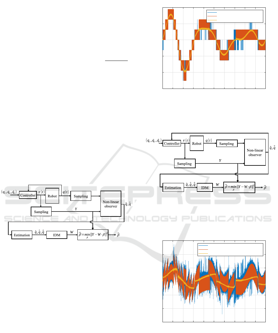
3.2 Identification
To mitigate the impact of noise on the identification
results when using the least squares method, we first
propose to compute the observation matrix W in (6)
using ( ˆq,
ˆ
˙q,
ˆ
¨q) as shown in Fig. 3, where ˆq and
ˆ
˙q are
the estimated joint position and velocity made using
the previously described nonlinear observer, while
ˆ
¨q
is the joint acceleration computed as a central differ-
ence derivative of
ˆ
˙q.
Figure 3: Least squares identification scheme of parameters
β considering noisy torque measurements Y and an observa-
tion matrix W computed using the inverse dynamic model
(IDM) with position ˆq and velocity
ˆ
˙q estimated using a non-
linear observer.
This method is always applicable regardless of the
system since it uses the measures on the system with-
out modifying the structure of the controller. On the
other hand, the PID control torque signal Y still re-
mains noisy due to the usage of the measured quan-
tized position at the controller input. Therefore, this
method cannot be used with the DIDIM approach,
which uses only the torque measurements, without
modification of the control structure.
In order to also reduce the torque noise, we pro-
pose to use the estimates ( ˆq,
ˆ
˙q) as PID controller in-
puts as shown in Fig. 5. In such a case, identification
results using LS and DIDIM techniques are expected
to be improved.
0 1 2 3 4 5 6 7 8 9 10
Time (s)
-15
-10
-5
0
5
10
Velocity (rad/s)
Measured velocity
Simulated quantized velocity
Simulated estimated velocity (EKF)
Figure 4: Comparison between measured velocity (blue),
simulated quantized velocity (orange) and estimated veloc-
ity using the proposed extended Kalman filter with 30% of
uncertainty on model parameters (yellow).
Figure 5: Least squares identification method of parameters
β considering torque Y computed using a modified control
structure integrating the non-linear observer, and an obser-
vation matrix W computed using the inverse dynamic model
(IDM) with position ˆq and velocity
ˆ
˙q estimated using this
non-linear observer.
0 1 2 3 4 5 6 7 8 9 10
Time (s)
-0.03
-0.02
-0.01
0
0.01
0.02
0.03
Torque (N.m)
Measured Torque
PID torque using quantized position
PID torque using estimated position (EKF)
Figure 6: Comparison between measured torque (blue),
simulated PID torque computed using quantized position
(orange) and simulated PID torque computed using position
estimated from the proposed extended Kalman filter with
30% of uncertainty on model parameters (yellow).
Contribution to Robot System Identification: Noise Reduction using a State Observer
699

4 METHOD VALIDATION
4.1 Experimental Setup
Simulations were carried out in Matlab and Simulink
environments to validate the suggested identification
approach, utilizing a 1 DOF system simulating the
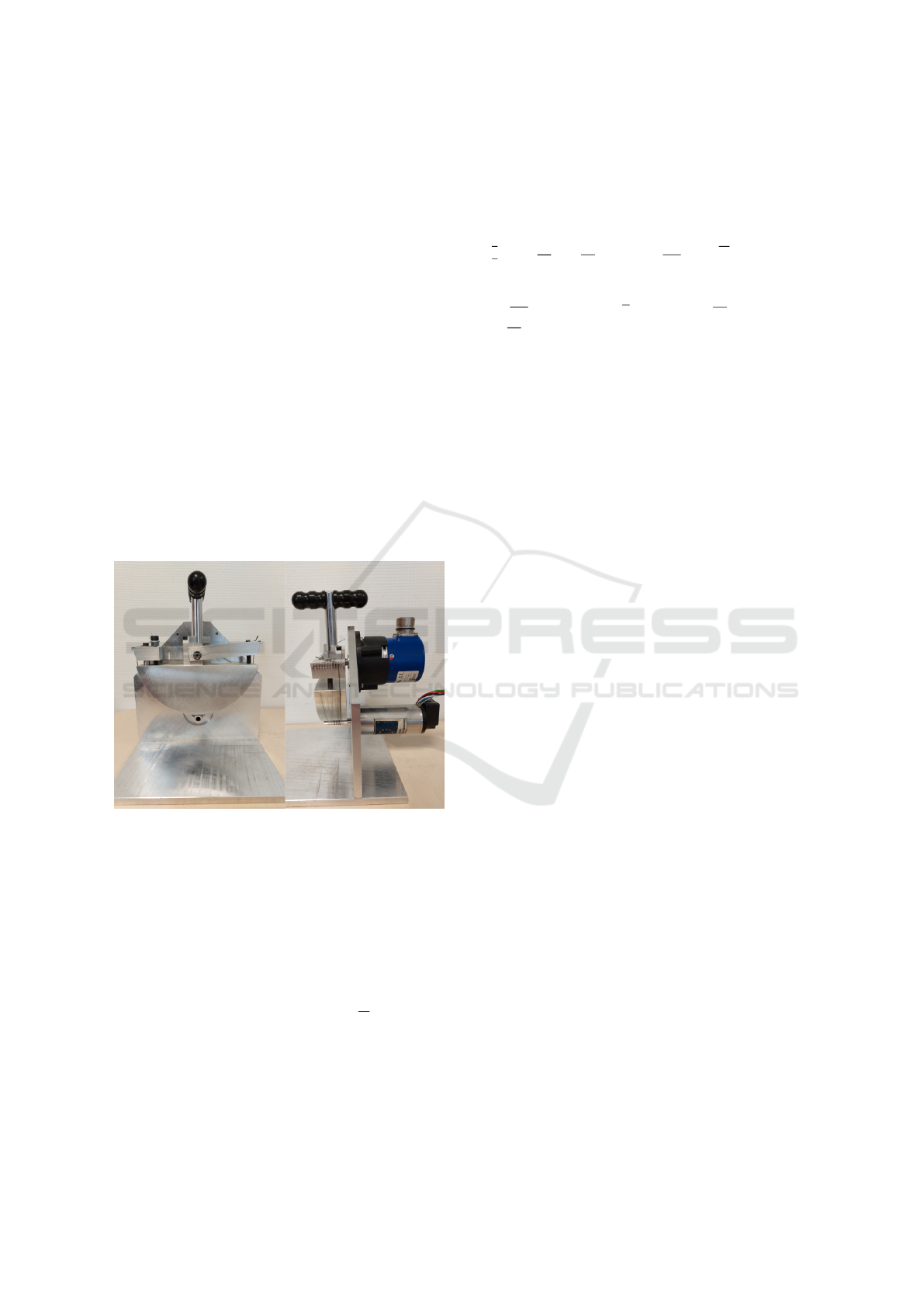
real system depicted in Fig. 7. Simulations are
chosen here since they provide the ground truth for
the confirmation of results. The actual system is
a cable-driven robot with a reduction ratio of 15.
It is made up of a handle and a mass linked by
a cable to a maxon motor (EC-max 40mm, brush-
less 120W, model 283871) with a HEDL 5540 en-
coder that measures the angular position of the motor
shaft. This encoder has a resolution of 500 counts
per turn, which corresponds to a quantization step
Q
quant
= 2π/(500 × 4) = 0.0031416 rad. A
PID controller implemented in an EPOS3 driver con-
nected to the maxon motor directly controls the sys-
tem. More details on the system’s conception and
structure can be found in (Dang, 2013).
Figure 7: Handle cable-driven system with a maxon mo-
tor (EC-max 40mm, brushless 120W, model 283871) and
a HEDL 5540 encoder with a resolution of 500 counts per
turn controlled by an EPOS3 controller, used as the simula-
tion’s reference.
4.2 Validation Scenario
In such a case, the IDM in (1) may be reduced to:
τ = J ¨q+F
v
˙q+F
c
sign( ˙q)+M
s
g cos(
q
N
+q
0
), (24)
where N is the reduction ratio, g is the gravity, q
0
is
the initial position of the motor shaft, M
s
∈ R is the
first moment, J ∈ R is the equivalent inertia of the
motor shaft and the handle, F
v
and F
c
∈ R are the fric-
tion coefficients defined in (2).
In this case, (19) can be written as follows:
x
k+1
=

q
k
˙q
k

+

˙q
k
1
ˆ
J

τ
k
−
ˆ
F
v
˙q
k
−
ˆ
F
c
sign( ˙q
k
) −
ˆ
M
s
gcos(
q
k
N
+ q
0
)


· T
s
,
(25)
with
ˆ
M
s
= (1 +w
1
)
ˆ
M
s
,
ˆ
J = (1+w
2
)
ˆ
J,
ˆ
F
v
= (1 +w
3
)
ˆ
F
v
and
ˆ
F
c
= (1 + w
4
)
ˆ
F
c
, where
ˆ
M
s
,
ˆ
J,
ˆ
F
v
and
ˆ
F
c
are the
estimations of M
s
,J, F
v
and F
c
respectively.
According to (23), the measurement noise covari-
ance matrix is set to R = (0.0031416)
2
/12 = 8.2247 ·
10
−7
, and the process noise covariance matrix is set to
Q = σ
2
w
· I
4
, i.e. the same relative trust level is given
to all parameters. By choosing σ
w
= 0.3, we con-
sider that our initial estimations of the parameters are
within an interval of 30% of their real value.
The initial value of the state is set to x
0
= [0 0]
T
,
as imposed by the excitation trajectory. The position
uncertainty of the covariance matrix P
0
is set to R,
which represents the uncertainty of the position sen-
sor, whereas the velocity uncertainty is set to 0.1 arbi-
trarily since it has influence only on the first iterations.
To evaluate the efficiency of our approach, we
compare different identification methods:
Method 1: LS with quantized data, without filtering
or observation (see Fig. 1).
Method 2: DIDIM with quantized data (see Fig. 2).
Method 3: LS with measured torque and estimated
position and velocity using the proposed EKF (see
Fig. 3).
Method 4: LS with torque computed from the po-
sition and velocity estimated using the proposed
EKF (see Fig. 5).
Method 5: DIDIM with torque computed from the
position and velocity estimated using the pro-
posed EKF.
4.3 Simulation Results and Discussions
Table 1 and Fig. 8 compare the identified parameters
and their standard deviations, obtained using methods
1-5 with the observer regulation provided in section
4.2, to the ground-truth values. We can observe that
the proposed methods 3 and 5 produce better identifi-
cation results than the conventional method 1.
Method 3 actually enhances the identification re-
sults by employing the estimated position and ve-
locity (as illustrated in Fig. 4) using the proposed
EKF, allowing LS to approach the performance of the
DIDIM technique defined in method 2 as well as the
ground-truth values. Furthermore, method 5 results
ICINCO 2022 - 19th International Conference on Informatics in Control, Automation and Robotics
700

Method 1 Method 2 Method 3 Method 4 Method 5
1.4
1.42
1.44
1.46
1.48
1.5
1.52
1.54
M
s
: First moment (Kg.m)
10
-3
Groundtruth
Method 1 Method 2 Method 3 Method 4 Method 5
0
0.5
1
1.5
2
2.5
J: Inertia (Kg.m
2
)
10
-5
Groundtruth
Method 1 Method 2 Method 3 Method 4 Method 5
0.4
0.6
0.8
1
1.2
1.4
1.6
1.8
F
v
: Viscous friction (N.m/rad/s)
10
-4
Groundtruth
Method 1 Method 2 Method 3 Method 4 Method 5
2.3
2.35
2.4
2.45
2.5
2.55
2.6
2.65
F
s
: Dry friction (N.m)
10
-3
Groundtruth
Figure 8: Comparison of identification results and standard deviation with respect to ground-truth values using the proposed
extended Kalman filter having as parameters the ground-truth values with 30% uncertainty on parameters.
Table 1: Comparison of identification results and standard
deviation using ideal extended Kalman filter with 30% un-
certainty on parameters.
M
s
(Kg.m) J(Kg.m
2
) F
v
(N.m/rad/s) F
s
(N.m)
Ground-truth 1.5187E-03 1.9046E-05 1.4500E-04 2.4790E-03
Method 1
1.4283E-03
± 1.3593E-05
1.7965E-06
± 1.2876E-08
6.3077E-05
± 1.0339E-05
2.5816E-03
± 4.4402E-05
Method 2
1.4996E-03
± 3.0773E-05
1.5579E-05
± 5.7634E-06
1.5510E-04
± 1.4790E-05
2.4275E-03
± 5.8413E-05
Method 3
1.4947E-03
± 2.1065E-05
1.2700E-05
± 3.9009E-07
1.1378E-04
± 1.4004E-05
2.5036E-03
± 5.4817E-05
Method 4
1.4521E-03
± 2.9487E-06
2.5303E-06
± 1.3379E-07
1.7448E-04
± 1.9369E-06
2.3262E-03
± 7.5778E-06
Method 5
1.4996E-03
± 2.6699E-06
1.6578E-05
± 5.0017E-07
1.5207E-04
± 1.2856E-06
2.4433E-03
± 5.0779E-06
generated by DIDIM with torque computed from the
estimated position and velocity using the proposed
EKF (as illustrated in Fig. 6) approach the ground-
truth values more closely than method 2 results ob-
tained by DIDIM with noisy torque, and have a lower
variance.
Method 4 doesn’t seem to improve identification
results as much as expected. This could be due to
the integration of the observer in the control structure.
This point should be investigated in future works.
5 CONCLUSIONS
This paper proposes a method for the identification
of the dynamic parameters of a robotic system. The
method uses an extended Kalman filter to estimate
the position and velocity of the system based on the
quantized position measurements. These estimates
are used as inputs to the controller, resulting in a
smoother torque output that can be used in the DIDIM
identification method. The formulation of the filter al-
lows an intuitive tuning based on known sensor char-
acteristics and on the confidence on the model param-
eter initial estimations. A simple, one degree of free-
dom system is used as an illustration for the validation
of the method. Simulation validation shows that the
proposed method improves the identification results.
Contribution to Robot System Identification: Noise Reduction using a State Observer
701

As future work we plan to validate the method on
the real system as well as on more complex systems.
Further study of the influence of the tuning of the ex-
tended Kalman filter will also be carried out to vali-
date the robustness of the proposed method.
REFERENCES
Akdo
˘
gan, E., Aktan, M. E., Koru, A. T., Selc¸uk Arslan, M.,
Atlıhan, M., and Kuran, B. (2018). Hybrid impedance
control of a robot manipulator for wrist and forearm
rehabilitation: Performance analysis and clinical re-
sults. Mechatronics, 49:77–91.
Atkeson, C. G., An, C. H., and Hollerbach, J. M. (1986).
Estimation of inertial parameters of manipulator loads
and links. The International Journal of Robotics Re-
search, 5:101–119.
Bogdan, I. C. (2010). Mod
´
elisation et commande
de syst
`
emes lin
´
eaires de micro-positionnement :
application
`
a la production de micro-composants
´
electroniques. PhD thesis, Universit
´
e Paul Verlaine
- Metz.
Brunot, M., Janot, A., Young, P., and Carrillo, F. (2018).
An improved instrumental variable method for indus-
trial robot model identification. Control Engineering
Practice, 74:107–117.
Dang, Q.-V. (2013). Conception et commande d’une in-
terface haptique
`
a retour d’effort pour la CAO. PhD
thesis, Universit
´
e Polytechnique Hauts-de-France.
Gautier, M. (1997). Dynamic identification of robots with
power model. In Proceedings of International Con-
ference on Robotics and Automation, volume 3, pages
1922–1927.
Gautier, M., Janot, A., and Vandanjon, P.-O. (2013). A new
closed-loop output error method for parameter iden-
tification of robot dynamics. IEEE Transactions on
Control Systems Technology, 21:428–444.
Han, Y., Wu, J., Liu, C., and Xiong, Z. (2020). An iterative
approach for accurate dynamic model identification
of industrial robots. IEEE Transactions on Robotics,
36:1577–1594.
Khalil, W. and Dombre, E. (2002). Chapter 9 - dynamic
modeling of serial robots. In Modeling, Identification
and Control of Robots, pages 191–233. Oxford.
Leboutet, Q., Roux, J., Janot, A., Guadarrama-Olvera, J. R.,
and Cheng, G. (2021). Inertial parameter identifica-
tion in robotics: A survey. Applied Sciences, 11.
Mayeda, H., Yoshida, K., and Osuka, K. (1990). Base
parameters of manipulator dynamic models. IEEE
Transactions on Robotics and Automation, 6:312–
321.
Olsen, M., Swevers, J., and Verdonck, W. (2002). Max-
imum likelihood identification of a dynamic robot
model: Implementation issues. The International
Journal of Robotics Research, 21:89–96.
Pham, M., Gautier, M., and Poignet, P. (2001). Identifica-
tion of joint stiffness with bandpass filtering. In Pro-
ceedings 2001 ICRA. IEEE International Conference
on Robotics and Automation, volume 3, pages 2867–
2872.
Shardt, Y. A., Yang, X., and Ding, S. X. (2016). Quantisa-
tion and data quality: Implications for system identi-
fication. Journal of Process Control, 40:13–23.
Swevers, J., Ganseman, C., Tukel, D., de Schutter, J., and
Van Brussel, H. (1997). Optimal robot excitation and
identification. IEEE Transactions on Robotics and Au-
tomation, 13:730–740.
ICINCO 2022 - 19th International Conference on Informatics in Control, Automation and Robotics
702