Simulation Study on Robot Calibration Approaches

Pavel Kozlov

and Alexandr Klimchik

Innopolis University, Innopolis, Russian Federation

Keywords:

Elastostatic Calibration, Industrial Robot, Robot Calibration, Identiﬁcation Method, Simulation, Models

Comparison.

Abstract:

The paper compares elastostatic calibration approaches for serial industrial robots. Speciﬁcally, this paper

compares identiﬁcation strategies based on the different measurement point locations and data fusion algo-

rithms. The paper analyzes several robot calibration hypotheses based on different robot models. All the

hypotheses were tested in a simulation study with 1000 data sets. The results showed that “4-6DoF after

6+3DoF” and “3+6DoF comb” methods demonstrated the best results for the considered methods. Strategies

were at least 1.86 times more accurate for the resulting deviation metric than the classical “6DoF” identiﬁca-

tion.

1 INTRODUCTION

Robots are widely used in assembling, welding, and

machining operations (Nubiola and Bonev, 2013; Wu

et al., 2015a; Qin et al., 2016). These operations

require high positioning accuracy during the techno-

logical processes (Park et al., 2012). Consequently,

the ﬁnal product accuracy is strictly dependent on the

robot accuracy. Therefore, a robot should be accurate

enough. Unfortunately, robots make position errors

which decreases the required accuracy. To solve this

issue, some calibration technique must be provided

(Li et al., 2021).

Robot calibration might be classiﬁed into geomet-

ric (Kamali and Bonev, 2019) and elastostatic calibra-

tion (Klimchik et al., 2017). Traditionally, positioning

errors are assumed to be mostly provided by geomet-

ric errors (Wu et al., 2015b; Elatta et al., 2004). These

errors are mainly introduced by links length and joint

offsets which are constant values. These values do not

depend on robot conﬁguration or any external load-

ing. The scientiﬁc community developed certain tech-

niques to reduce such errors and almost ignore any ge-

ometric factors (Daney and Emiris, 2001; Driels et al.,

1993; Veitschegger and Wu, 1987; Hage, 2012; Ren-

ders et al., 1992).

Another source of errors are the elastostatic prob-

lems. These problems arise during any technological

process and depend on robot conﬁguration and ex-

https://orcid.org/0000-0002-7582-3517

https://orcid.org/0000-0002-2244-1849

ternal load (Ma et al., 2017). Elastostatic errors ap-

pear in addition to the geometrical ones and may have

higher impact on the resulting accuracy on differ-

ent operations, milling for instance (Klimchik et al.,

2016). Nevertheless, these errors can be also reduced.

The reduction might be done by selecting an appropri-

ate model and error compensation approach (Nguyen

et al., 2022; Klimchik et al., 2014; Gonzalez et al.,

2022).

From our experience, model parameters have dif-

ferent impact on the positioning accuracy (Klimchik

et al., 2015). Therefore we can reduce the model

to achieve robot accuracy with lower model com-

plexity (Mamedov et al., 2018). Importantly, such a

model must have only signiﬁcant parameters (Klim-

chik et al., 2015). Numerous research might help to

reduce model complexity within required robot cali-

bration accuracy (Joubair et al., 2012; Jin and Gans,

2015).

This paper mainly aims to study different strate-

gies for elastostatic calibration. The study was based

on several measurement point locations, such as on

the end-effector, after the second joint, on the robot

arm, and after the forth joint. Selecting several mea-

surement points might give some additional possibil-

ities for robot calibration. To enhance the validity of

presented analysis, we are comparing two different in-

dustrial robots. These robots have different joint com-

pliance to analyze the suggested identiﬁcation strate-

gies in details. Hence, their joints have different im-

pacts on the resulting accuracy and require additional

investigation.

516

Kozlov, P. and Klimchik, A.

Simulation Study on Robot Calibration Approaches.

DOI: 10.5220/0011321800003271

In Proceedings of the 19th International Conference on Informatics in Control, Automation and Robotics (ICINCO 2022), pages 516-523

ISBN: 978-989-758-585-2; ISSN: 2184-2809

2 PROBLEM STATEMENT

In this work, the simulation study was based on the

serial industrial manipulator Kuka KR-270 R-2700

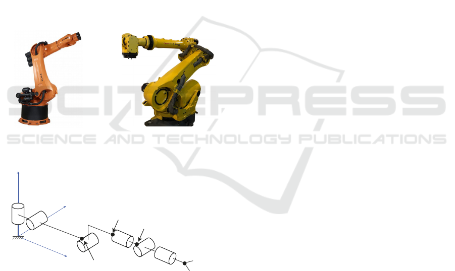
and Fanuc r2000ic 165F (Fig. 1). These manipulators

have similar kinematics structures but different joint

compliance and link lengths (Klimchik et al., 2017).

Basically, the classical identiﬁcation is based on mea-

suring points on the end-effector. The classical ap-

proach can calibrate all parameters at once. Unfor-

tunately, the classical identiﬁcation does not allow to

identify joint parameters separately and may lead to

a mutual balancing of the errors in the identiﬁed pa-

rameters. To overcome this limitation, we introduced

and analysed several new measurement points. This

analysis allowed us to decouple robot parameters and

calibrate them more accurately (Jiang et al., 2020). In

our study, both robots contained four reference points

corresponding to different kinematics models: 2DoF,

3DoF, 4DoF and 6DoF (full) (see Fig. 2).

(a) Kuka KR-270 R-2700.

(b) Fanuc r2000ic 165F.

Figure 1: Robots under study.

full

short

2 DoF

4 DoF

Figure 2: Equivalent kinematics scheme of a serial indus-

trial robot.

These points theoretically allow us to identify sep-

arately parameters of robot joint elasticity. In addi-

tion, these points also may achieve additional bene-

ﬁts. Therefore, we tested the following identiﬁcation

strategies:

1. 6DoF. The identiﬁcation algorithm considered

the full kinematics (T

f ull

) and identiﬁed full vec-

tor of elastic parameters c at once. This algorithm

required the data from the robot conﬁguration q

measured position of the end-effector p

f ull

and

the values of applied wrenches w

2. 6DoF after 3DoF. At the ﬁrst step, we identiﬁed

the ﬁrst three elements of vector c using three DoF

kinematics. At the second step, we used vector c

as the initial condition and identiﬁed full vector

c (wrist elasticity) using full kinematics. This al-

gorithm required the data from the robot conﬁg-

uration q

, measured position for the three DoF

kinematics p

3 DoF

and end-effector p

f ull

, as well

as the values of applied wrenches w

3. 4-6DoF after 3DoF. At the ﬁrst step, we identi-

ﬁed the ﬁrst three elements of vector c using three

DoF kinematics. At the second step, we identi-

ﬁed the last three elements of vector c using the

full kinematics. This algorithm required the data

from the robot conﬁguration q

, measured posi-

tion for the 3 DoF kinematics p

3 DoF

and end-

effector p

f ull

, as well as the values of applied

wrenches w

4. 6DoF after 3+3DoF. The identiﬁcation algorithm

considered the kinematics (T

f ull

) and identiﬁed

the full vector of elastic parameters c at once. This

algorithm used the vector c from “4-6DoF after

3DoF” strategy as initial condition for calibration.

This algorithm required the data from the robot

conﬁguration q

, measured position for the three

DoF kinematics p

3 DoF

and end-effector p

f ull

, as

well as the values of applied wrenches w

5. 3+6DoF comb. The identiﬁcation algorithm con-

sidered the full kinematics (T

f ull

) and three DoF

kinematics (T

3 DoF

) simultaneously. Selected

kinematics is used to identify the full vector of

elastic parameters c at once. This algorithm re-

quired the data from the robot conﬁguration q

measured position for the three DoF kinematics

3 DoF

and end-effector p

f ull

, as well as the val-

ues of applied wrenches w

6. 4-6DoF after 6+3DoF. The identiﬁcation algo-

rithm considered the full kinematics (T

f ull

) and

identiﬁed the last three elements of vector of elas-

tic parameters c at once. This algorithms used the

full vector c from “3DoF + 6DoF comb” strategy

as initial condition for calibration. The algorithm

required the data from the robot conﬁguration q

measured position for the three DoF kinematics

3 DoF

and end-effector p

f ull

, as well as the val-

ues of applied wrenches w

7. 3-6DoF after 2DoF. At the ﬁrst step, we identi-

ﬁed the ﬁrst two elements of vector c using two

DoF kinematics. At the second step, we identi-

ﬁed the last four elements of vector c using the

Simulation Study on Robot Calibration Approaches

517

full kinematics (T

f ull

). This algorithm required

the data from the robot conﬁguration q

, measured

position for the two DoF kinematics p

2 DoF

and

end-effector p

f ull

, as well as the values of applied

wrenches w

8. 5-6DoF after 4DoF. At the ﬁrst step, we identi-

ﬁed the ﬁrst four elements of vector c using four

DoF kinematics. At the second step, we iden-

tify last two elements of vector c using the full

kinematics (T

f ull

). This algorithm required the

data from the robot conﬁguration q

, measured

position for the four DoF kinematics p

4 DoF

and

end-effector p

f ull

, as well as the values of applied

wrenches w

However, it is not clear which strategy will

achieve the most accurate robot model parameters

identiﬁcation and the highest robot precision accuracy

after calibration. What is more, it is not evident how

the selected model and its reduction effect the cali-

bration accuracy. Hence, let us formulate several re-

search questions which we addressed in this study.

RQ1: How does the model complexity affect the

identiﬁcation accuracy?

RQ2: How should we determine and introduce mea-

surement points?

RQ3: Which number of reference point location for

different kinematics models is able to achieve

the accurate robot model parameters identiﬁ-

cation and the highest robot precision accu-

racy after calibration?

RQ4: How should we evaluate the efﬁciency of elas-

tostatic calibration?

During this work every strategy was validated by

1000 different initial random seed conﬁguration. The

results present mean values along with all different

initial random seed conﬁgurations. Moreover, we

compared the described strategies for different noise

both for position and orientation values. This noise

was randomly normal (Gaussian) distributed noise

without any shift of its mean. We also conducted sev-

eral experiments with different standard deviation val-

ues: 0 m (or rad), 5 ∗ 10

−5

m (or rad), 1 ∗ 10

−4

m (or

rad), 2 ∗ 10

−4

m (or rad) and 5 ∗ 10

−4

m (or rad). We

selected such noise value based on robot parameters,

especially repeatability. This value was about 60 µm

for the selected robots. The noise value was also con-

nected with measurement system accuracy, for exam-

ple, a laser tracker had an accuracy of about 16 µm.

Therefore, the selected noise was going to validate the

identiﬁcation approaches with similar noise impact as

experimental validation on the real system.

For every robot conﬁguration during simulation

analysis, we applied the randomly generated force

(|F| = 1000 N) with a randomly generated direction.

The force application point was shifted by 0.5 m

along the Y axis. This offset was required to identify

the last joint stiffness.

3 BENCHMARK EXAMPLE

The experiments were based on the “KUKA KR-270

R-2700” and “Fanuc R2000ic-165F” industrial ma-

nipulators. They both have similar kinematics scheme

(see Fig. 2). Its 6DoF or full (T

f ull

), 2DoF kinematics

2 DoF

), 3DoF kinematics (T

3 DoF

) and 4DoF kine-

matics (T

4 DoF

) can be computed as follows:

2 Do f

= T

base

tool

(1)

3 Do f

= T

∗

2 Do f

tool

(2)

4 DoF

= T

∗

3 Do f

tool

(3)

f ull

= T

∗

4 DoF

tool

(4)

where q

is the value of i

joint, θ

is the value

of i

virtual joint, l

represents i

link length and

, R

, T

are elementary homoge-

neous transformation matrices. The matrices T

∗

2 Do f

∗

3 Do f

, T

∗

4 Do f

represent matrices T

2 Do f

, T

3 Do f

4 Do f

respectively without tool transformation. Here

tool

,( j ∈ {2,3,4,6}) describe measurement points

transformations, T

base

describes the base transforma-

tion. For simplicity, during the experiments T

base

and

tool

were equal to identity matrix.

Any identiﬁcation technique requires Jacobian

matrices concerning the set of unknown parameters.

The Jacobians concerning virtual joint variables θ was

computed using Screw Theory (Jazar, 2022) for all

models in this study.

Furthermore, we should describe the parameters

of the robot. Both robots had similar kinematic struc-

tures and elastostatic models. They had different links

length and equivalent joint compliances (see Table 1

for details). We selected robots with a similar struc-

ture to compare their difference in calibration accu-

racy.

4 IDENTIFICATION

PROCEDURE

First, we selected an elastostatic model of a serial

manipulator (Klimchik et al., 2017). So, we had to

ICINCO 2022 - 19th International Conference on Informatics in Control, Automation and Robotics

518

Table 1: Equivalent joint compliances.

Robot

joint compliances, µm/N

Kuka 0.54 0.29 0.42 2.79 3.48 2.07

Fanuc 1.23 0.37 0.46 2.68 2.70 2.72

choose from several modeling approaches: Matrix

Structural Analysis (MSA), Finite Elements Analy-

sis (FEA), and Virtual Joint Modeling (VJM). Their

advantages and disadvantages have been presented

many times (Pashkevich et al., 2009; Deblaise et al.,

2006; Quennouelle and Gosselin, 2008; Piras et al.,

2005; Chen and Kao, 2000; Marie et al., 2013). Here,

we chose the VJM modeling since it used the most

appropriate method for the considered problem. In

VJM modeling, the manipulator was presented as a

sequential of rigid and elastic components: a ﬁxed

“Base”, several ﬂexible actuated joints “Ac”, some

ﬂexible “Links” and an “End-effector”. According to

this method, the model of every link had to be ex-

tended by adding six DoF springs. We also had to

add one DoF spring for every joint (Dumas et al.,

2011; K

ovecses and Angeles, 2007; Klimchik et al.,

2012). Fig. 3 describes the elasticity of the related

links/joints. Additionally, we extended the reduced

VJM model only by adding one DoF spring after ev-

ery joint.

Base

Link 1

Link 6 Tool. . .

1-d.o.f

spring

6-d.o.f

spring

6-d.o.f

spring

Figure 3: VJM scheme of the robot.

With this method, every link was represented as a

thick-walled beam. What is more, we had to extend

the robot kinematics transformation by adding T

1−6

where T

1−6

is computed as follows:

1−6

= T

(5)

Generally, this model contained numerous vari-

ables that cannot be strictly identiﬁed. Hence, we

had to use the reduced VJM model. According to

this technique, the rigid model had to be extended

by adding one DoF spring followed by every joint as

shown in Fig. 3.

The robot deﬂection depended on the conﬁgura-

tion q, while the applied wrench w of the serial ma-

nipulator for the given conﬁguration was computed as

follows

w = K

δt (6)

where K

is the Cartesian stiffness matrix, δt is the

end-effector deﬂection (Salisbury, 1981; Klimchik

et al., 2014).

The virtual joints displacement was found by the

following equation:

θ = K

−1

w (7)

where J

is the Jacobian matrix with respect to virtual

joints θ that depends on the conﬁguration q and K

the aggregated spring stiffness matrix of the size 6×6.

This matrix describes the elastostatic properties of the

manipulator links/joints.

To generate a simulation dataset, we used the

above method. Here, wrench direction was randomly

computed, but the applied force was constant (|F| =

1000 N). Using computed θ and robot kinematics

transformation we determined the ideal robot posi-

tion (p

init

) which all identiﬁcation strategies should

achieve. Here, all required values were computed and

the dataset might be stored.

In practice, K

matrix was unknown and had

to be found by any identiﬁcation technique. Basi-

cally, identiﬁcation required a dataset with several

measured conﬁgurations, points, and applied wrench.

Therefore, we can write the elastostatic model for the

experiment as

δt

= J

θ,i

−1

θ,i

(8)

where, δt

is end-effector displacement in the i

ex-

periment and w

is corresponding external wrench ap-

plied to the manipulator end-effector. The elastostatic

model can be rewritten to show the connection be-

tween known and unknown parameters as follows:

δt

= A

c (9)

where the vector c collects all unknown compliance

coefﬁcients and

= [J

i,1

i,2

,.. .,J

i,m

] (10)

Here J

i, j

represents columns of the Jacobian matrix

θ,i

= [J

i,1

i,2

,.. .,J

i,n

The identiﬁcation approach can be represented as

the optimization problem based on the calibration re-

quires several experiments. The solution of the de-

scribed problem can be represented as follows:

c = (

∑

i=1

)

−1

(

∑

i=1

δt

) (11)

where n is the number of experiments.

5 ANALYSIS

To compare the described algorithms, let us introduce

that the resulting K

was computed by mean comput-

ing along 1000 experiments per dataset length (ds):

= diag(k

) (12)

Simulation Study on Robot Calibration Approaches

519

(a) KUKA robot (b) Fanuc robot

Figure 4: Noise impact analysis for the 6DoF identiﬁcation strategy.

where diagonal element contains identiﬁed stiffness

values for each robot joint. To describe the accuracy

of computed parameters and taking into account that

we know ideal values, it is more indicative to compare

parameters in percent:

δk

comp

− k

init

∗ 100% (13)

where k

init

is initial robot joint stiffness. Unfortu-

nately, some values might be decoupled along with

joints stiffness identiﬁcation when joints were allo-

cated along the same axis. Hence, to neglect this

problem the result combined into single value:

∑

i=1

δk

(14)

The following identiﬁcation strategies results were

compared with respect to computed single value k

∑

Another method to compare considered strategies

was achieved by deviation comparison.

dev(ds) = mean(

1000

∑

i=1

(p(ds)

comp

− p(ds)

init

))

(15)

where ds is current dataset length value, p(ds)

comp

is computed end-effector position after selected cal-

ibration strategy, p(ds)

init

is initial simulated end-

effector position before calibration. The presented

metric dev(ds) will be able to analyze more important

metric such as resulting robot accuracy. Initial devi-

ations are presented in Table 2 for both robots before

any calibration technique. What is more, “Kuka ex-

tended” contained the deviation results for the Kuka

robot where the full VJM model was used during

dataset generation.

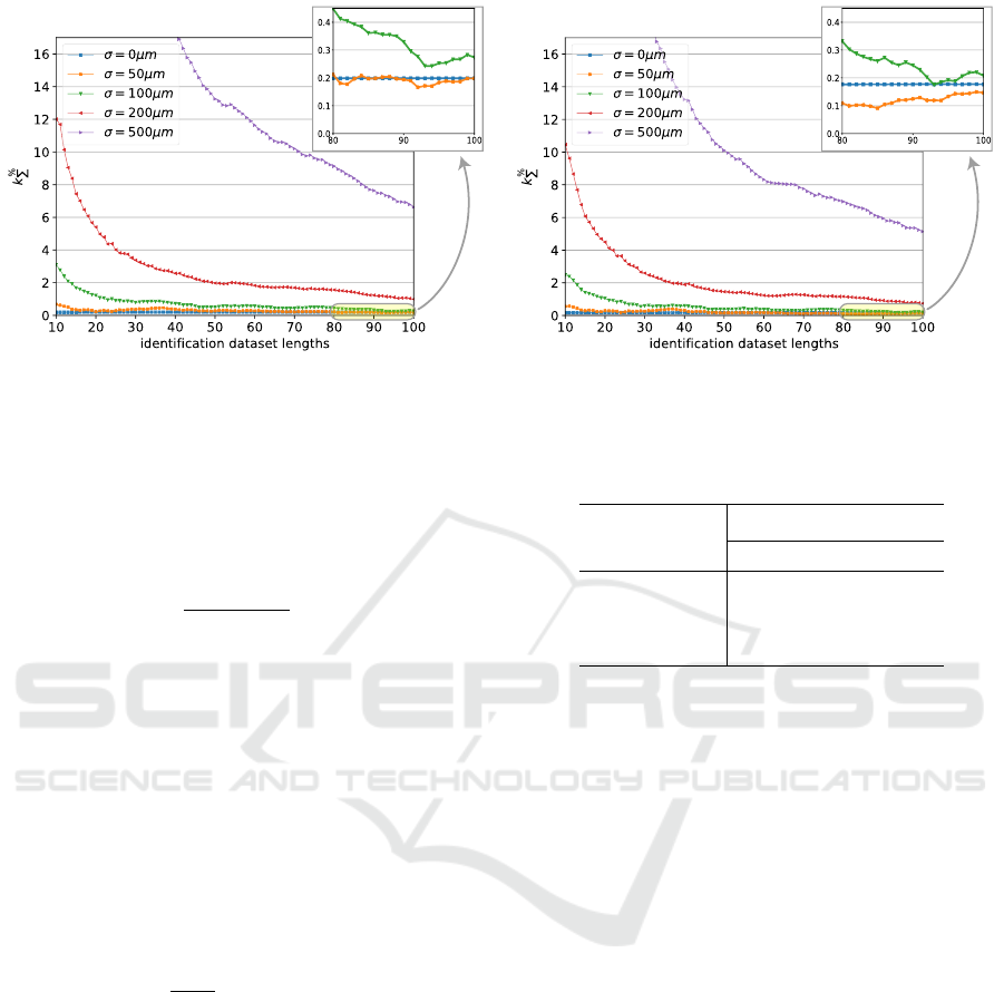
Firstly, we had to select the most representable

noise value. Fig. 4 demonstrates the achieved calibra-

tion results for the 6DoF identiﬁcation strategy along

Table 2: Initial end-effector deviation value for both robots

before calibration.

Robot

accuracy, mm

mean std max

Kuka 0.929 0.636 2.864

Fanuc 1.497 1.487 9.516

Kuka extended 1.749 1.116 4.743

with different noise values for both robots. The val-

ues of 0 µm, 50 µm and 100 µm demonstrated similar

results which tend to zero. Hence, their selection was

not representable to compare different identiﬁcation

strategies. Otherwise, 500 µm noise demonstrated a

lot of impacts from this noise. Hence, 500 µm noise

value did not tend to appropriate robot calibration re-

sults. Therefore, the following comparison was done

concerning 200 µm noise value. The classical 6DoF

strategy can achieve identiﬁcation accuracy of less

than 2 µm for both robots with less than 50 conﬁg-

urations in the dataset. This result is less than robot

repeatability, hence, it will produce a lower impact on

robot positioning accuracy.

Secondly, 6DoF, 6DoF after 3DoF and 6DoF af-

ter 3+3DoF strategies demonstrates the same results.

They were able to achieve the following joint compli-

ance with 20 conﬁgurations in the dataset presented in

Table 3. Generally, 6DoF strategy seemed to achieve

the result under any default conditions, no matter

which initial stiffness matrix selected, and which ini-

tial thetas had been chosen.

Table 4 and Fig. 5 demonstrate the comparison of

the achieved calibration results for the selected noise.

These metrics were able to demonstrate that 4-6DoF

after 6+3DoF strategy was more accurate for both

robots for any metric. 3+6DoF comb strategy was

able to achieve similar robot precision as the previous

ICINCO 2022 - 19th International Conference on Informatics in Control, Automation and Robotics

520

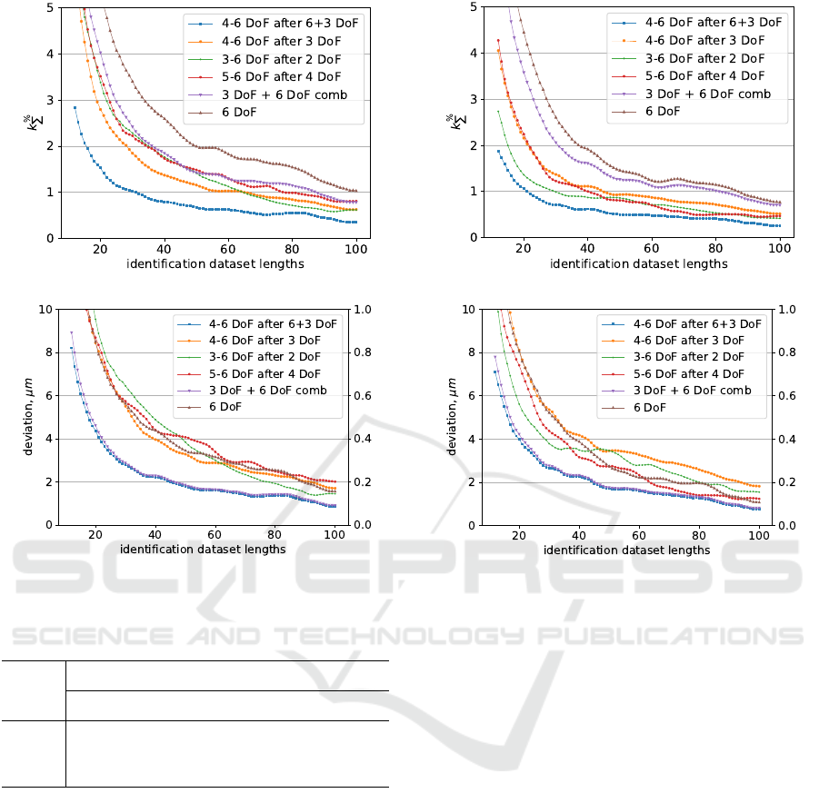
(a) Joint stiffness persantage difference for KUKA robot

(b) Joint stiffness persantage difference for Fanuc robot

(d) Resulting deviation mean value for Fanuc robot

Figure 5: Achieved results comparison for the noise 200 µm for robot calibration identiﬁcation strategies.

Table 3: Achieved joint compliances values, µm/N.

Robot

joint compliances, µm/N

Kuka 0.538 0.287 0.414 2.774 3.464

2.047

Fanuc 1.233 0.370 0.455 2.663 2.667

2.694

one. The 4-6DoF after 6+3DoF and 3+6DoF comb

identiﬁcation strategies were at least 1.86 times more

accurate for the resulting deviation metric than the

classical 6DoF identiﬁcation. Unfortunately, 3+6DoF

comb strategy produced 2.75 times less precise re-

sults for exact joint compliance calibration than 4-

6DoF after 6+3DoF strategy. Other strategies’ re-

sults were strictly dependent on the selected robot.

The 3-6DoF after 2DoF strategy could calibrate the

Fanuc robot exact joint compliance within 30 con-

ﬁgurations, but this strategy was not so accurate for

the Kuka robot. During these comparisons, the Fanuc

robot achieved more accurate results for any metric

than the Kuka robot.

We also compared how residuals parameters had

been affected by the robot precision after any cali-

bration. This experiment was done for Kuka robots

modeling. The resulting accuracy was lower than

366 µm for any identiﬁcation strategy with the noise

of 200 µm. Therefore, the residuals parameters had a

lot of impact on the resulting robot accuracy and se-

lecting appropriate number or residual parameters re-

quired to have an accurate robot model. In this case,

acceptable results could also be achieved.

Despite the beneﬁts, the developed approaches

had certain limitations. Firstly, different robots did

not achieve similar results. This problem required

analyzing how robot model parameters such as joint

compliance and any geometrical parameters were in-

ﬂuenced by the resulting robot accuracy (Klimchik

et al., 2017; Klimchik and Pashkevich, 2017).

Secondly, the robot conﬁgurations were selected

randomly. Optimal selection of measurement poses

might increase resulting robot accuracy. Optimal se-

lection of measurement poses does not have a lot of

impact on results because all experiments were done

with 1000 iterations. Hence, identiﬁcation strategies

were compared more clearly.

Simulation Study on Robot Calibration Approaches

521

Table 4: Comparison analysis for the noise 200 µm for robot calibration identiﬁcation strategies.

Strategy Robot

Metric

∑

(20), % k

∑

= 1% dev(20), µm dev = 2µm

4-6DoF after 6+3DoF

Kuka 1.471 31 4.229 45

Fanuc 1.036 22 3.867 46

4-6DoF after 3DoF

Kuka 2.743 66 8.206 90

Fanuc 2.107 46 7.860 95

3-6DoF after 2DoF

Kuka 3.411 65 9.594 77

Fanuc 1.379 30 5.592 80

5-6DoF after 4DoF

Kuka 3.485 76 8.680 100

Fanuc 2.175 39 7.332 64

3+6DoF comb

Kuka 4.049 87 4.507 46

Fanuc 3.633 82 4.143 46

6DoF

Kuka 5.405 100 8.386 89

Fanuc 4.494 87 7.921 72

∑

(20) demonstrates how precise exact joint compliance values can be achieved with 20 conﬁgurations.

∑

= 1% demonstrates how many conﬁgurations are required to achieve quite accurate joint

compliance values. In this case robot should achieve not more that 1% for k

∑

metric.

dev(20) demonstrates how accurate robot precision can be achieved with 20 conﬁgurations.

dev = 2µm demonstrates how many conﬁgurations are required to achieve robot precision less than 2 µm.

6 CONCLUSION

The paper presents the simulation study on robot cal-

ibration approaches. Several new assumptions were

tested while the analysis. The achieved results led to

the following conclusions concerning the formulated

hypothesis:

1. Selecting an appropriate model affects the identi-

ﬁcation accuracy. The reduced model was able to

compensate 80% of joint and link elasticity. In the

case if link elasticity is negligibly small the model

was able to compensate 99% of compliance er-

rors. The presented comparison was made for 20

measurement conﬁgurations in the dataset. There-

fore, selecting an appropriate model can increase

robot accuracy more precisely.

2. Select additional points which are visible during

experimental validation demonstrated more accu-

rate results. The exact point location requires ad-

ditional study because of the tendency that point

location depends on robot parameters.

3. We discovered that combining several datasets

during identiﬁcation is able to achieve more ac-

curate results. This result is caused by partially

increasing the dataset used for identiﬁcation. In

particular, we used two-point position measures

instead of one point for every conﬁguration.

4. The robot accuracy may be measured through

several metrics. Mostly, the results coincided

with different metrics. The exact metric selec-

tion strictly depends on the required task. Nev-

ertheless, the comparison of resulting robot end-

effector displacement might be the primary way to

evaluate the efﬁciency of elastostatic calibration.

In the future, the developed methodology will

be focused on comparing geometric and elastostatic

robot parameter to analyze how the robot parameters

inﬂuence the resulting calibration accuracy.

ACKNOWLEDGEMENTS

This work was supported by Russian Scientiﬁc Foun-

dation (Project number 22-41-02006).

REFERENCES

Chen, S.-F. and Kao, I. (2000). Conservative congruence

transformation for joint and cartesian stiffness matri-

ces of robotic hands and ﬁngers. I. J. Robotic Res.,

19:835–847.

ICINCO 2022 - 19th International Conference on Informatics in Control, Automation and Robotics

522

Daney, D. and Emiris, I. (2001). Robust parallel robot cal-

ibration with partial information. volume 4, pages

3262–3267.

Deblaise, D., Hernot, X., and Maurine, P. (2006). A system-

atic analytical method for pkm stiffness matrix calcu-

lation. pages 4213 – 4219.

Driels, M., Swayze, W., and Potter, S. (1993). Full-pose

calibration of a robot manipulator using a coordinate-

measuring machine. The Inter. J. of Advanced Manu-

facturing Technology, 8:34–41.

Dumas, C., Caro, S., Garnier, S., and Furet, B. (2011). Joint

stiffness identiﬁcation of six-revolute industrial serial

robots. Robot. Comput.-Integr. Manuf., 27:881–888.

Elatta, A., Gen, L., Zhi, F., Daoyuan, Y., and Fei, L. (2004).

An overview of robot calibration. Information Tech-

nology J., 3:74–78.

Gonzalez, M. K., Theissen, N. A., Barrios, A., and

Archenti, A. (2022). Online compliance error com-

pensation system for industrial manipulators in con-

tact applications. Robot. Comput.-Integr. Manuf.,

76:102305.

Hage, H. (2012). Identiﬁcation and physical simulation of

a st

aubli tx90 robot during high-speed milling.

Jazar, R. (2022). Theory of Applied Robotics: Kinematics,

Dynamics, and Control (3rd Edition). Springer.

Jiang, Z., Huang, M., Tang, X., and Song, B. (2020).

Observability index optimization of robot calibration

based on multiple identiﬁcation spaces. Autonomous

Robots, 44:1029–1046.

Jin, J. and Gans, N. (2015). Parameter identiﬁcation for in-

dustrial robots with a fast and robust trajectory design

approach. Robot. Comput.-Integr. Manuf., 31:21–29.

Joubair, A., Slamani, M., and Bonev, I. (2012). Kinematic

calibration of a ﬁve-bar planar parallel robot using all

working modes. Robot. Comput.-Integr. Manuf., 29.

Kamali, K. and Bonev, I. (2019). Optimal experiment de-

sign for elasto-geometrical calibration of industrial

robots. IEEE/ASME Trans. on Mech., 24:2733–2744.

Klimchik, A., Ambiehl, A., Garnier, S., Furet, B., and

Pashkevich, A. (2016). Experimental study of robotic-

based machining. IFAC-PapersOnLine, pages 174–

179.

Klimchik, A., Ambiehl, A., Garnier, S., Furet, B., and

Pashkevich, A. (2017). Efﬁciency evaluation of

robots in machining applications using industrial per-

formance measure. Robot. Comput.-Integr. Manuf.,

48:12–29.

Klimchik, A., Bondarenko, D., Pashkevich, A., Briot, S.,

and Furet, B. (2014). Compliance error compensation

in robotic-based milling. Informatics in Control, Au-

tomation and Robotics, 283.

Klimchik, A., Furet, B., Caro, S., and Pashkevich, A.

(2015). Identiﬁcation of the manipulator stiffness

model parameters in industrial environment. Mech.

Mach. Theory, 90:1–22.

Klimchik, A. and Pashkevich, A. (2017). Serial vs. quasi-

serial manipulators: Comparison analysis of elasto-

static behaviors. Mech. Mach. Theory, 107:46–70.

Klimchik, A., Pashkevich, A., Caro, S., and Chablat, D.

(2012). Stiffness matrix of manipulators with passive

joints: Computational aspects. Robot. IEEE Trans. on,

28:955–958.

ovecses, J. and Angeles, J. (2007). The stiffness matrix in

elastically articulated rigid-body systems. Multibody

System Dynamics, 18:169–184.

Li, Z., Li, S., and Luo, X. (2021). An overview of calibra-

tion technology of industrial robots. IEEE/CAA J. of

Automatica Sinica, 8:23–36.

Ma, L., Bazzoli, P., Sammons, P., Landers, R., and Bristow,

D. (2017). Modeling and calibration of high-order

joint-dependent kinematic errors for industrial robots.

Robot. Comput.-Integr. Manuf., 50.

Mamedov, S., Popov, D., Mikhel, S., and Klimchik, A.

(2018). Compliance error compensation based on re-

duced model for industrial robots. pages 190–201.

Marie, S., Courteille, E., and Maurine, P. (2013). Elasto-

geometrical modeling and calibration of robot manip-

ulators: Application to machining and forming appli-

cations. Mech. Mach. Theory, 69:13–43.

Nguyen, V. L., Kuo, C.-H., and Lin, P. T. (2022). Compli-

ance error compensation of a robot end-effector with

joint stiffness uncertainties for milling: An analytical

model. Mech. Mach. Theory, 170:104717.

Nubiola, A. and Bonev, I. (2013). Absolute calibration of

an abb irb 1600 robot using a laser tracker. Robot.

Comput.-Integr. Manuf., 29:236–245.

Park, I.-W., Lee, B.-J., Cho, S.-H., Hong, Y.-D., and

Kim, J.-H. (2012). Laser-based kinematic calibra-

tion of robot manipulator using differential kinemat-

ics. Mech. IEEE/ASME Trans. on, 17:1059–1067.

Pashkevich, A., Chablat, D., and Wenger, P. (2009). Stiff-

ness analysis of overconstrained parallel manipula-

tors. Mech. Mach. Theory, 44:966–982.

Piras, G., Cleghorn, W., and Mills, J. (2005). Dynamic

ﬁnite-element analysis of a planar high-speed, high-

precision parallel manipulator with ﬂexible links.

Mech. Mach. Theory, 40:849–862.

Qin, J., L

eonard, F., and Abba, G. (2016). Real-time tra-

jectory compensation in robotic friction stir welding

using state estimators. IEEE Trans. on Control Sys-

tems Technology, 24:2207–2214.

Quennouelle, C. and Gosselin, C. (2008). Stiffness Matrix

of Compliant Parallel Mechanisms, pages 331–341.

Springer.

Renders, J.-M., Rossignol, E., Becquet, M., and Hanus, R.

(1992). Kinematic calibration and geometrical param-

eter identiﬁcation for robots. Robot. and Automation,

IEEE Trans. on, 7:721 – 732.

Salisbury, J. (1981). Active stiffness control of a manipu-

lator in cartesian coordinates. volume 1, pages 95 –

100.

Veitschegger, W. and Wu, C.-h. (1987). A method for cali-

brating and compensating robot kinematic errors. vol-

ume 4, pages 39 – 44.

Wu, L., Yang, X., and Chen, K. (2015a). A minimal poe-

based model for robotic kinematic calibration with

only position measurements. IEEE Trans. on Automa-

tion Science and Eng., 12:758–763.

Wu, Y., Klimchik, A., Caro, S., Furet, B., and Pashkevich,

A. (2015b). Geometric calibration of industrial robots

using enhanced partial pose measurements and design

of experiments. Robot. Comput.-Integr. Manuf., 35.

Simulation Study on Robot Calibration Approaches

523