Structural Damage Localization via

Deep Learning and IoT Enabled Digital Twin

Marco Parola

, Federico A. Galatolo

, Matteo Torzoni

, Mario G. C. A. Cimino

and Gigliola Vaglini

Department of Information Engineering, University of Pisa, Largo L. Lazzarino 1, Pisa, Italy

Department of Civil and Environmental Engineering, Politecnico di Milano, Piazza L. da Vinci 32, Milano, Italy

Keywords: Convolutional Neural Network, IoT, Digital Twin, Structural Health Monitoring.

Abstract: Structural Health Monitoring (SHM) of civil structures using IoT sensors is a major emerging challenge. SHM

aims to detect and identify any deviation from a reference condition, typically a damage-free baseline, to keep

track of the relevant structural integrity. Machine Learning (ML) techniques have recently been employed to

empower vibration-based SHM systems. Supervised ML can provide more information than unsupervised

ML, but it requires human intervention to appropriately label data describing the nature of the damage.

However, labelled data related to damage conditions of civil structures are often unavailable. To overcome

this limitation, a key solution is a Digital Twin relying on physics-based numerical models to simulate the

structural response in terms of the vibration recordings provided by IoT devices during the events of interest,

such as wind or seismic excitations. This paper presents such comprehensive approach to address the damage

localization task by exploiting a Convolutional Neural Network (CNN). Early experimental results related to

a pilot application involving a sample structure, show the potential of the proposed approach and the

reusability of the trained system in presence of varying loading scenarios.

1 INTRODUCTION AND

BACKGROUND

All structures, whether buildings, bridges, oil and gas

pipelines, are subject to several external actions and

sources of degradation that might compromise their

structural performance. This can happen due to a

faulty construction process, lack of quality control, or

unexpected loadings, environmental actions and

natural hazards such as earthquakes. In order to

observe the resulting changes in the structure, and to

quickly react before a major damage occurs, it is

crucial to implement an autonomus damage

identification system. Systematic diagnostic and

prognostic activities allow for timely maintenance

and repair actions, with a direct impact on reducing

operating costs. In the last years, increasingly

sophisticated Structural Health Monitoring (SHM)

https://orcid.org/0000-0003-4871-4902

https://orcid.org/0000-0001-7193-3754

https://orcid.org/0000-0002-1031-1959

https://orcid.org/0000-0003-1949-6504

systems have been developed. These systems

constantly measure structural responses to load

solicitations and perform different tasks, such as

damage detection, localization, quantification and

estimation of the impact of environmental effects on

the building (Ye, Jin, & Yun, 2019). A SHM

architecture consists of different layers. In the lowest

layer, a sensor network is installed on the structure

and collects vibrational and environmental data. The

upper layers deal with communication and data

storage. In the analysis layer, the algorithms solving

SHM tasks are implemented. Finally, in the highest

layer the results of these computations are displayed

via reports or web platforms.

Recently, many Machine Learning (ML)

vibration-based strategies have been proposed to

solve different SHM problems. SHM systems based

on ML algorithms are increasingly popular because

of their ability to capture damage-sensitive patterns

Parola, M., Galatolo, F., Torzoni, M., Cimino, M. and Vaglini, G.

Structural Damage Localization via Deep Learning and IoT Enabled Digital Twin.

DOI: 10.5220/0011320600003277

In Proceedings of the 3rd International Conference on Deep Learning Theory and Applications (DeLTA 2022), pages 199-206

ISBN: 978-989-758-584-5; ISSN: 2184-9277

199

that traditional algorithms often fail to detect (Wang,

2022). In particular, using Supervised Learning (SL),

the ML system models a relationship based on input-

output pairs, whereas Unsupervised Learning (UL)

finds patterns in the input data that are provided

without a corresponding output label. In structural

engineering, a dominant method of UL is the

Frequency Domain Decomposition (FDD), used for

Modal Analysis (MA). Specifically, MA studies the

dynamic properties of the systems in the frequency

domain. MA uses the overall mass and stiffness of a

structure to find the periods at which it naturally

resonates (Rainieri, Fabbrocino, & Cosenza, 2007).

The outputs of MA are frequency response, modal

shapes and damping. FDD consists of two main steps:

(i) frequency detection and (ii) tracking. Frequency

detection is performed periodically by clustering

algorithms, in order to find frequencies that have

occurred since the previous execution. In the tracking

phase, the frequencies found are combined to create

trends describing the overall properties of the

structure and how they change over time (Fabio,

Ferrari, & Rizzi, 2016).

UL methods detect anomalies or drifts in the

inputs, without providing a clear and explicit

explanation. In order to get explicit information such

as damage location, quantification and type, data

enriched with labels and SL methods are adopted

(Wang, 2022). However, dealing with civil structures,

labeled data related to different environmental

conditions or seismic events are often unavailable. To

overcome this limitation, a key solution is a Digital

Twin (DT) reproducing both structural physics-based

numerical models and input vibrations provided by

IoT devices during the events of interest, such as wind

or seismic forces (Aydemir, Zengin, & Durak, 2020).

A DT consists of three components: a physical

structure in the real world, a digital model of the

structure in a computerized environment, and the

integration of data and information that tie the virtual

and real products together (David, Chris, Aydin,

Jason, & Ben, 2020). For a successful DT

implementation, all related assets need to be properly

defined in order to collect the necessary data. Indeed,

since data modeling and simulation have a non-

negligible cost, efficient tools and methods are

needed. The process in which these tools are defined

and the DT is implemented is called digital

transformation. An important method of the digital

representation of the structure based on computerized

tools, is called Finite Element (FE). FE numerically

solves differential equations of structural

https://www.movesolutions.it/deck/

engineering. Since the computational cost associated

to the solution of such numerical models can easily

become prohibitive, in view of a systematic

evaluation for dataset generation purposes a Model

Order Reduction (MOR) strategy is adopted to

computationally speed up the construction of the

necessary data (Rosafalco, Torzoni, Manzoni, &

Mariani, 2021). Subsequently, Supervised Deep

Learning (DL) models can be created with the

generated data, to solve specific SHM tasks.

This paper shows the overall methodology and a

pilot application in the field, based on a

Convolutional Neural Network (CNN) performing

the damage localization task on a sample structure.

Early experimental results show the potential of the

proposed approach, as well as the reusability of the

trained system on varying environmental actions.

The paper is structured as follows. Section 2

covers material and methods, whereas experimental

results and discussions are covered by Section 3.

Finally, Section 4 draws conclusions and future work.

2 MATERIALS AND METHODS

The SHM methodology applied in this work consists

of two main parts: (i) the design and implementation

of the DT used as dataset generator to create a dataset

that reflects realistic environmental effects; (ii) the

damage localization problem via a supervised DL

architecture. Finally, an analysis of the performance

of the DL model is presented, considering different

loading conditions (Yuqian, Chao, Kevin, Huiyue, &

Xun, 2020).

2.1 Digital Twin Development

To faithfully represent a real scenario through a DT,

three aspects are considered: (i) physics-based model

of the structure to be monitored, (ii) the digital

reproduction of low-intensity seismic loads, and (iii)

the introduction of noise components affecting the

IoT sensor networks. The representation of the

physical aspects involves the modeling of the

building and the simulation of a sensor system for the

vibrational IoT data acquisition. Let us consider, in

Figure 1, a pilot example of building to monitor. A

commercial example of IoT system is represented in

Figure 2: a Deck – Dynamic Displacement Sensor

. It

is a mono-axial wireless device, which acquires

displacements with an accuracy of 0.01 mm, suitable

for dynamic monitoring.

DeLTA 2022 - 3rd International Conference on Deep Learning Theory and Applications

200

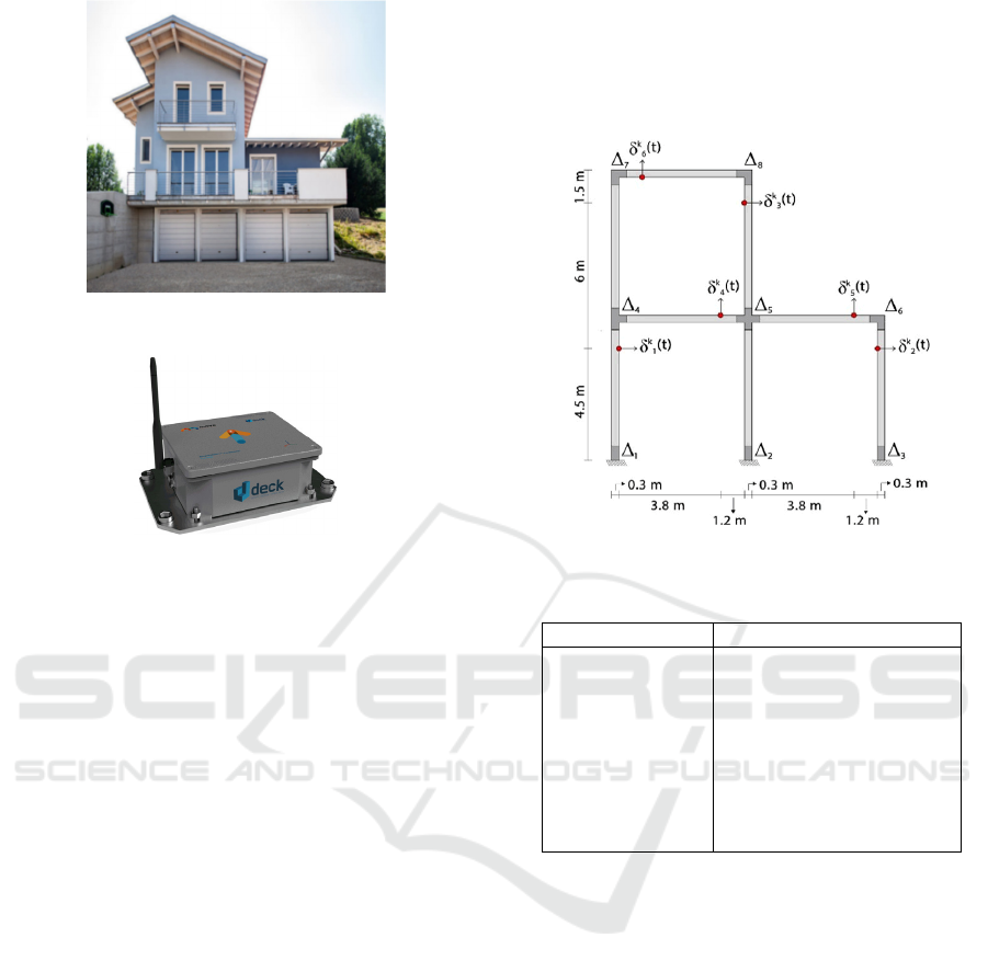
Figure 1: A pilot example of building to monitor.

Figure 2: An example of IoT device: Deck – Dynamic

Displacement Sensor © Move Srl, Italy.

To clearly represent the methodology, a

simplified DT will be illustrated in the following for

the sake of significance. Figure 3 shows a simplified

representation of the DT of the building. Here, the

building is modeled as a two-dimensional (2D) frame,

assuming a plane stress formulation; the geometry has

been discretized in 3450 constant strain triangle finite

elements. In order to reduce the computational burden

of the data generation process, the structural model,

which is based on the FE method, is replaced by a

Reduced-Order Model (ROM) (Torzoni, Rosafalco,

& Manzoni, 2020)

Overall, N

=6 synchronized

vibrational sensor devices, with sampling rate 25Hz,

have been considered to collect displacements

measurements. Each displacement measure δ

(t) has

been prefixed in terms of direction

(vertical/horizontal) and orientation (up/right). The

bottom edges are assumed perfectly clamped to the

ground. The output damage scenarios ∆

have been

limited to 9 classes, located on related dark grey areas

in Figure 3, and defined in Table 1. Here, the essential

assumption is the presence of only one damage

location after a seismic event. As a consequence, only

a discrete number N

∆

of damage scenarios are defined

based on mechanical response, loading conditions,

and aging processes. In the DT, damage is modeled

as a localized reduction of stiffness on the selected

regions.

An important aspect concerns the synchronization

between IoT devices, which is a critical requirement

for system operation. Implementing a

synchronization mechanism in a real-world scenario

is not a zero-cost process. Several protocols can be

adopted to guarantee this requirement, depending on

the system type (Yiğitler, Behnam, & Riku, 2020).

Figure 3: A simplified Digital Twin representation.

Table 1: Output damage scenarios.

Damage class Location description

∆

Undamaged

∆

Ground floor – left

∆

Ground floor – mid

∆

Ground floor – right

∆

floor - left

∆

floor - mid

∆

floor - right

∆

Roof - left

∆

Roof - mid

Another important aspect concerns the input

loading condition to which the structure is subject to.

In this work, low intensity seismic loads are

considered; Ground Motion Prediction Equations

(GMPE) adapted from (Paolucci, et al., 2018)

(Sabetta & Pugliese, 1996) have been adopted to

faithfully reproduce this aspect. The main advantage

of GMPE is the ability to generate spectrum-

compatible accelerograms as a function of: local

magnitude Q, epicentral distance R, and site geology.

The following ranges have been considered: Q ∈(4.8,

5.3); R ∈(80, 100) km; rocky conditions. The

parameters

and R have been modelled by uniform

probability density functions.

A vibration record is then generated by evaluating

the model of the structure under the seismic event k.

It consists of displacement measurements δ

(t) of

fixed length L=1750, δ

(t) ∈

ℝ

and refers to a time

period ∆t=70s. An event is detected and recorded by

Structural Damage Localization via Deep Learning and IoT Enabled Digital Twin

201

all N

sensors, yielding a seismic event observation

(t) ∈ℝ

⨯

, i=0,…,N

Given an observation δ

(t) related to a seismic

event k, a damage class Δ

∈ℕ is assigned to it,

therefore, a record of our dataset D is defined as a pair

[δ

, ∆

], i=0,…,N

. In Table 1 the N

=9 damage

scenarios included the undamaged baseline state,

labeled as d=∆

A damage level l

∈ℝ is also associated with

each event, to represent the intensity of the stiffness

reduction involving the subdomain that is related to

∆

; l

is sampled by a uniform probability density

function in the range ∈(0.05, 0.25).

The iterative process of simulating the structural

response for varying parameters values is repeated for

=9999 times D ∈ℝ

⨯

2.2 The Seismic Events Dataset

The influence of a generic signal δ

(.)

on a system can

be measured by computing its power 

(.)

as shown

in Equation (1). Different components have been

considered to model the various aspects influencing

the sensed data, such as traffic, temperature, pressure,

rain, wind, and so on. (Joaquín, Ana, Jesús, &

Fernando, 2015). All these components contribute to

produce the environmental phenomena that affect the

behaviour of the structure.

To measure the quantity of all components in the

signal, a metric has been defined, i.e., the

Environmental Condition (EC). EC is defined as the

ratio of the power of a seismic signal 



and the

power of environmental noise 



. In order to avoid

large values to skew the plot, a logarithmic scale has

been applied, computing the EC metric in decibels as

shown in Equation (2). An EC higher than 1 (higher

than 0 dB) denotes more seismic signal than

environmental noise, whereas a ratio equal to infinity

indicates that the environmental noise is equal to zero.

In this paper, the environmental noise introduced

during the training phase is Gaussian, producing

EC=10dB.



(.)

δ

(.)











(1)

=10









(2)

Both seismic signal and environmental noise

powers must be measured at the same or equivalent

points in a system, and within the same system

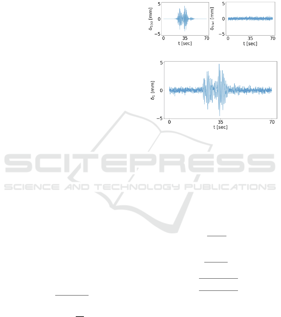
bandwidth. Figure 4 shows an example of seismic,

environmental signals, together with the integrated

signal.

(a)

(b)

(c)

Figure 4: (a) example of seismic signal detected by sensor

1 during the simulation of seismic events; (b) example of

environmental noise modelling traffic, temperature,

pressure, rain, wind, and so on; (c) the integrated signal.

Data preprocessing has been carried out to

manage the scaling of the data. In particular, a z-score

scaling has been applied for all signals collected from

the same sensor.

More formally, Equations (3), (4) and (5) define

the preprocessing.













−







(3)





















(4)













−















(5)

To split the data into training (90%) and test

(10%) sets, the hold-out method is adopted; the

relevant class numerosity for training and test sets is

summarized in Table 2.

DeLTA 2022 - 3rd International Conference on Deep Learning Theory and Applications

202

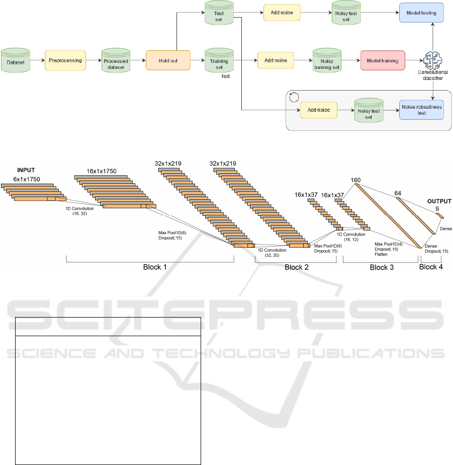
Figure 5: Data Pipeline.

Figure 6: Convolutional NN architecture.

Table 2: Seismic events dataset composition.

Label Training set Test set

∆

994 117

∆

1003 108

∆

1008 103

∆

998 113

∆

992 119

∆

1001 110

∆

998 113

∆

1005 106

∆

1001 110

2.3 The CNN Architecture

To summarize the data pipeline, Figure 5 shows the

main steps. A Convolutional Neural Network (CNN)

is proposed to perform such classification task. CNN

is a class of NNs that has become dominant in various

domains such as computer vision, signal processing,

speech recognition (Li, Zhang, Zhang, & Wei, 2017)

(Galatolo F. A., 2018) (Galatolo F. A., 2019).

CNN is designed to automatically and adaptively

learn feature hierarchies through backpropagation,

using multiple building blocks such as convolution

layers, pooling layers, and fully connected layers.

This section focuses on the CNN architecture,

illustrated in Figure 6. Specifically, the convolutional

architecture consists of 4 blocks. The first three deal

with feature extraction, whereas the last one performs

the classification task. Each of the first three blocks

consists of a 1D convolutional layer, a 1D max

pooling layer, and a dropout layer; in addition, a

flatten layer is added at the end of the feature

extractor. The classifier block is composed of two

dense layers separated by a dropout one.

Figure 6 shows the hyper parameter values for the

design of each layer. The training is run for 200

epochs, using the Adam optimization algorithm; the

validation set is generated from the training set by

taking 20% of the records.

To avoid overfitting phenomena, an early

stopping condition callback is set. It ends the CNN

training before it has reached the number of allowed

epochs, when the loss computed on the validation set

does not decrease for a number of epochs equal to

patience=10.

The damage location task is modelled as a

multiclass classification problem, where the output

label to be predicted identifies a potential region on

the building. The categorical crossentropy is the loss

function to be minimized during training, used in

multiclass classification tasks. Equation (6) shows

how the loss function can be computed given an

Structural Damage Localization via Deep Learning and IoT Enabled Digital Twin

203

observation, where ∆′

is the i-th scalar target value in

the actual vector ∆′ obtained by transforming the

numerical variable ∆ into a categorical one; ∆



′

is the

corresponding value in the predicted output.

=−∆′



∆



′







(6)

In order to measure the performances of the

model, three metrics are adopted, accuracy, precision,

and recall, represented in Equation (7), (8) and (9)

respectively.



=

+

+ ++

(7)

=



+

(8)

=



+

(9)

where TP = True Positive, FP = False Positive, TN

= True Negative, and FN = False Negative.

3 EXPERIMENTAL RESULTS

AND DISCUSSION

The overall methodology has been developed on

Google Colab (Bisong, 2019), a free platform based

on the open-source Jupyter project. Both the data

source and the code have been publicly released

(Parola, 2022), to foster collaboration and application

on various infrastructures.

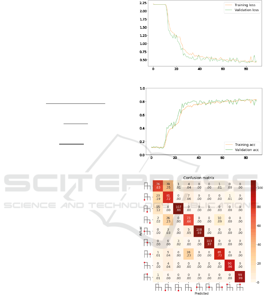
The device used is an NVIDIA Tesla K80 GPU.

The training process ends after 97 epochs due to early

stopping condition, restoring model weights from the

end of the best epoch.

The loss and accuracy on the validation set during

training are shown in Figure 7 and Figure 8,

respectively. From both figures, we can observe that

there are no overfitting phenomena, the curves

computed on training and validation sets have the

same trend. Moreover, we can observe a slightly

irregular trend, due to the presence of dropout layers.

The convolutional model achieves a global

accuracy of 83%. Figure 9 shows the accuracies

through a confusion matrix, while Table 3 shows the

precision and recall values per class.

Figure 7: Loss learning curve.

Figure 8: Accuracy learning curve.

Figure 9: Confusion matrix on test set.

Since the environmental noise level may vary, and

this is not known a priori, an assessment of the model

performance with different noise level of the test set

is carried out, to understand its robustness with

respect to different environmental conditions. Model

testing is repeated 13 times, varying the noise level

and producing the corresponding EC values of the test

set between 1 dB and 25 dB, as shown in Figure 10.

DeLTA 2022 - 3rd International Conference on Deep Learning Theory and Applications

204

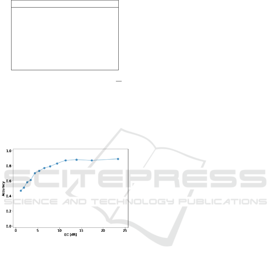
Table 3: Damage localization test results by class.

Class Precision Recall

∆

.56 .59

∆

.54 .61

∆

.95 .88

∆

.61 .71

∆

.94 .92

∆

.99 .97

∆

.91 .78

∆

1.0 .98

∆

1.0 1.0

In Figure 10, we can observe that the

convolutional model is still able to detect damage-

sensitive patterns, despite the increasing amount of

noise in the data. Specifically, by using training data

with EC= 10 dB, good performance is achieved on

test set with EC larger than 10 dB. For test set with

EC lower than 10 DB a decrease in the accuracy value

can be observed. In this application context, the

prediction capability of the damage location is

acceptable as long as the EC value is larger than 5 dB.

Figure 10: Model accuracy on test set varying the EC

values.

4 CONCLUSIONS

In this work, an integrated method made by a

Convolutional Neural Network and a Digital Twin

has been proposed in the context of Structural

Damage Localization. To illustrate the approach, the

Digital Twin of a sample infrastructure is modelled

through a Reduced-Order Model method, together

with the digital model of commercial IoT devices.

The CNN architecture has been also detailed. The

overall pipeline has been developed and publicly

released. Different environmental conditions have

been experimented on testing, to show the

effectiveness of the approach.

This paper represents a preliminary work to show

the potential of the proposed approach. As a future

work, other problem to solve, such as building

affected by simultaneous multiple damages, should

be considered. Further, acceleration sensing should

be taken into account together with displacement, to

support a multimodal monitoring.

ACKNOWLEDGEMENTS

This work has been supported by: (i) the TLC

company Move Srl, Lucca LU, Italy; (ii) a research

team of Politecnico di Milano composed by Alberto

Corigliano, Andrea Manzoni, Luca Rosafalco and

Stefano Mariani; (iii) the Italian Ministry of

Education and Research (MIUR) in the framework of

the CrossLab project (Departments of Excellence).

REFERENCES

Aydemir, H., Zengin, U., & Durak, U. (2020). The digital

twin paradigm for aircraft review and outlook. In AIAA

Scitech 2020 Forum (p. 0553).

Bisong, E. (2019). Bisong, E. (2019). Building machine

learning and deep learning models on Google cloud

platform. Berkeley, CA, USA.

David, J., Chris, S., Aydin, N., Jason, Y., & Ben, H. (2020).

Characterising the Digital Twin: A systematic literature

review. CIRP Journal of Manufacturing Science and

Technology, 29, 36-52.

Fabio, P., Ferrari, R., & Rizzi, E. (2016). Output-only

modal dynamic identification of frames by a refined

FDD algorithm at seismic input and high damping.

Mechanical Systems and Signal Processing, 265-291.

Galatolo, F. A. (2018). Using Stigmergy to Incorporate the

Time into Artificial Neural Networks. Springer, Cham,

pp. 248-258.

Galatolo, F. A. (2019). Using stigmergy as a computational

memory in the design of recurrent neural networks.

arXiv preprint, arXiv:1903.01341.

Joaquín, A., Ana, J., Jesús, U., & Fernando, J. Á. (2015).

Realistic modeling of underwater ambient noise and its

influence on spread-spectrum signals. OCEANS 2015-

Genova, (pp. 1-6) IEEE.

Li, D., Zhang, J., Zhang, Q., & Wei, X. (2017).

Classification of ECG signals based on 1D convolution

neural network. In 2017 IEEE 19th International

Conference on e-Health Networking, Applications and

Services (Healthcom), (pp. 1-6). IEEE.

Paolucci, R., Gatti, F., Infantino, M., Smerzini, C., Özcebe,

A. G., & Stupazzini, M. (2018). Broadband ground

motions from 3D physicsbased numerical simulations

using artificial neural networks. Bulletin of the

Seismological Society of America, 108(3A), 1272-

1286.

Structural Damage Localization via Deep Learning and IoT Enabled Digital Twin

205

Parola, M. (2022). structural_health_monitoring. Tratto da

GitHub:

github.com/MarcoParola/structural_health_monitoring

Rainieri, C., Fabbrocino, G., & Cosenza, E. (2007).

Automated Operational Modal Analysis as structural

health monitoring tool: theoretical and applicative

aspects. p. 479-484.

Rosafalco, L., Torzoni, M., Manzoni, A., & Mariani, S.

(2021). Online structural health monitoring by model

order reduction and deep learning algorithms.

Computers & Structures, 255, 106604.

Sabetta, F., & Pugliese, A. (1996). Estimation of response

spectra and simulation of nonstationary earthquake

ground motions. Bulletin of the Seismological Society

of America, 86(2), 337-352.

Torzoni, M., Rosafalco, L., & Manzoni, A. (2020). A

Combined Model-Order Reduction and Deep Learning

Approach for Structural Health Monitoring under

Varying Operational and Environmental Conditions.

Engineering Proceedings, 2(1), 94.

Wang, X. (2022). Probabilistic machine learning and

Bayesian inference for vibration-based structural

damage identification. Tratto da Polyu electronic

theses: theses.lib.polyu.edu.hk

Ye, X., Jin, T., & Yun, C. (2019). A review on deep

learning-based structural health monitoring of civil

infrastructures. Smart Struct. Syst.

Yiğitler, H., Behnam, B., & Riku, J. (2020). Overview of

time synchronization for IoT deployments: Clock

discipline algorithms and protocols. Sensors, 20(20),

5928.

Yuqian, L., Chao, L., Kevin, I.-K. W., Huiyue, H., & Xun,

X. (2020). Digital Twin-driven smart manufacturing:

Connotation, reference model, applications and

research issues. Robotics and Computer-Integrated

Manufacturing, 61, 101837.

DeLTA 2022 - 3rd International Conference on Deep Learning Theory and Applications

206