Generating a Multi-fidelity Simulation Model Estimating the Models’

Applicability with Machine Learning Algorithms

Christian Hürten

, Philipp Sieberg

and Dieter Schramm

Chair of Mechatronics, University of Duisburg-Essen, 47057 Duisburg, Germany

Keywords: Simulation, Model Fidelity, Multi-fidelity Model, Computational Effort, Machine Learning, Support Vector

Machine, Neural Network.

Abstract: Having access to large data sets recently gained increasing importance, especially in the context of automation

systems. Whether for the development of new systems or for testing purposes, a large amount of data is

required to satisfy the development goals and admission standards. This data is not only measured from

real-world tests, but with growing tendency generated from simulations, facing a trade-off between

computational effort and simulation model fidelity. This contribution proposes a method to assign individual

simulation runs the simulation model that has the lowest computation costs while still being capable of

producing the desired simulation output accuracy. The method is described and validated using support vector

machines and artificial neural networks as underlying vehicle simulation model classifiers in the development

of a lane change decision system.

1 INTRODUCTION

Over the last years, the availability of large data sets

has gained increasing importance in both research and

system development. Especially in the field of

automation, the demand for appropriate data is rising

as machine learning algorithms are receiving more

attention.

A popular application area for automation is the

automotive sector with its driver assistance systems

ranging from supportive systems like the lane

departure warning system to fully autonomous

driving vehicles. Even with classical controller

strategies and thus without the use of data-driven

algorithms, in the development process an exhaustive

amount of test cases has to be covered. Many of those

tests are nowadays performed in simulations.

(Paulweber, 2017)

On the one hand, the simulation-based testing

offers economic advantages. Depending on the

simulation environment, the test can be performed

faster than real-time, thus the development process

can be shortened. Furthermore, occurring system

failures do not harm testing personal nor real

https://orcid.org/0000-0002-6762-8877

https://orcid.org/0000-0002-4017-1352

https://orcid.org/0000-0002-7945-1853

hardware and can be eliminated before deployment in

expensive real-world prototypes. On the other hand,

tests in simulation environments come with practical

advantages. The tests can be carried out under

constant, deterministic environmental conditions,

which can be chosen independently of i.e. weather

impacts that real-world testing has to cope with.

(Sovani et al., 2017)

Other than providing an environment to test

developed systems, simulations can also be used in

the design process. Systems based on data-driven

machine learning algorithms need plenty of data to be

trained on. Whereas this data can be collected in the

real-world, using simulation data offers again a less

time and cost consuming alternative.

Using a simulation, the two important

characteristics are the underlying model’s fidelity and

the required computational resources. In general, the

more accurate the simulation model has to be, the

more computational power respective time is needed

for simulation.

While a complex simulation model may result in

highly accurate data for all regarded simulated events,

its complexity may not be necessary in each of these

Hürten, C., Sieberg, P. and Schramm, D.

Generating a Multi-ﬁdelity Simulation Model Estimating the Models’ Applicability with Machine Learning Algorithms.

DOI: 10.5220/0011318100003274

In Proceedings of the 12th International Conference on Simulation and Modeling Methodologies, Technologies and Applications (SIMULTECH 2022), pages 131-141

ISBN: 978-989-758-578-4; ISSN: 2184-2841

131

events. For some cases, a less complex model can be

sufficient in accuracy as well, whilst requiring less

computational resources.

As the trade-off between computational

requirements and model fidelity is not only subject to

automation system simulation but rather a general

problem in the field of simulations, many researchers

are investigating possible solutions, combining

multiple simulation models of varying fidelity to so-

called multi-fidelity models.

In (Fernandez-Godino et al., 2017), the authors

review different merging strategies for those multi-

fidelity models. E.g., the merging can be performed

by correcting the output of low fidelity models.

Therefore, the deviation from a high fidelity model is

analysed at given points, in the application this

deviation is estimated. (Biehler et al., 2015)

An alternative approach defines selection criteria

for each of the simulation models. This contribution

belongs to the latter strategy, the proposed method

uses a selection criterion per investigated model that

is learned from the models’ simulation data using

machine learning algorithms.

In the following, a short introduction into the

fundamentals of the used vehicle models and machine

learning algorithms is given. Afterwards, the

simulation framework is presented. Subsequently, the

proposed method is described before finally being

applied to the development of an automated lane

change decision system.

2 FUNDAMENTALS

This section presents an overview on the

fundamentals of the used vehicle models as well as

support vector machines and neural networks

2.1 Vehicle Dynamics

In this contribution, the simulations are performed

with four vehicle models. With increasing model

fidelity, those models are a point mass model, a linear

single-track model and two nonlinear single-track

models. Vehicle models with higher fidelity like a

dual-track model or a multi-body system are not

considered in this paper, since the focus of this work

is the presentation of the method determining the

required model fidelity. Furthermore, the performed

simulation does not include highly dynamical events

with high lateral accelerations and thus the single-

track models are sufficient to model the vehicles

dynamics accurately.

2.1.1 Point Mass Model

For the vehicle model with the lowest fidelity a point

mass model is used. The model uses the first order

Euler method to compute the vehicles position 𝒙 and

speed 𝒗 at discrete time intervals Δ𝑡 based on the

current acceleration 𝒂:

𝒙



𝑡Δ𝑡



𝒙



𝑡



𝒗



𝑡Δ𝑡



∙Δ𝑡

(1)

𝒗



𝑡Δ𝑡



𝒗



𝑡



𝒂



𝑡



∙Δ𝑡

(2)

In this model, neither rotational movement around

any axis nor tire characteristics are modelled.

(Alvarez Lopez et al., 2018)

2.1.2 Linear Single-Track Model

The linear single-track model is an often-used vehicle

simulation model describing the lateral behaviour of

a vehicle. For low lateral accelerations, this model is

very accurate but because of linearisation of the

equations, the model’s fidelity decreases with

increasing lateral accelerations.

The model does not include longitudinal forces,

thus only constant velocities can be simulated. The

only rotation allowed for this model is around the

vertical axis, the other rotations are restricted. Tire

modelling is done by a linear model depending on the

lateral slip angle and the cornering stiffness of the

tires. A detailed explanation of the model can be

found in many literature sources, e.g. in (Heißing &

Ersoy, 2011).

2.1.3 Nonlinear Single-Track Model

The highest fidelity models used in this work are

nonlinear single-track models. In general, this model

is modelling the movement in lateral and longitudinal

direction as well as the rotation around the vertical

axis. Considering the longitudinal component of the

model, an engine model is incorporated in

conjunction with resistance force modelling.

The vehicle-road contact point is modelled by the

empirical magic formula model, a nonlinear tire

model after (Pacejka, 2012). Since the equations of

this model are not linearized, the model does not

suffer from the accuracy loss for higher lateral

acceleration the linearized model has to deal with.

Optionally, this model can be complemented by a

roll and pitch model. Those models are linear models

of the rotational behaviour around the horizontal

axes. As those rotations are described by linear

models, they are only feasible for small rotational

movement. For further description of the nonlinear

single-track model and the roll model, please consider

SIMULTECH 2022 - 12th International Conference on Simulation and Modeling Methodologies, Technologies and Applications

132

(Schramm et al., 2018). The pitch model is described

in (Sieberg et al., 2019).

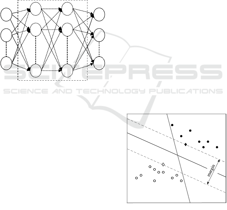
2.2 Artificial Neural Networks

The artificial neural networks (ANNs) considered in

this work are so-called fully-connected feedforward

neural networks. The signal flow in such ANNs is

always directed from the input-neurons through the

hidden neuron layers to the output neurons. Thereby,

every neuron of one layer – excluding the input layer

– is connected to all neurons of the preceding layer.

Figure 1 shows the structure of these ANNs,

exemplary with two hidden layers.

Figure 1: Fully-connected feedforward neural network with

two hidden layers.

In each neuron, its N inputs 𝒙∈ℝ



– hence the

outputs of the previous layer with N neurons inside –

are summed up with each input weighted by the

neuron’s weights 𝒘∈ℝ



. This sum is adjusted by

the neuron’s bias 𝑏∈ℝ to compensate for a possible

offset before the output of the neuron is calculated by

applying an activation function f



: ℝ→ℝ. Thus,

each neuron’s output 𝑦 can be described by:

𝑦f



𝒘



𝒙𝑏

(3)

Popular activation functions are the Tanh and

Sigmoid functions as well as the Exponential Linear

Unit (ELU) which is defined as follows:









x , x0

𝛼∙𝑒



1, x0

(4)

Thereby, the parameter 𝛼 describes the lower bound

of the function’s output. (Gron, 2017)

During the training of the ANN, the trainable

parameters weight and bias of the neurons are adapted

to fit the network to the given data. This is achieved

by the method of error backpropagation. Based on a

loss function, the difference between network output

and target output on the training data points is

computed. The error loss is then propagated

backwards through the ANN, from the output layer to

the input layer. During this backpropagation, the

gradients of the weights and biases are computed with

respect to the loss. These gradients are then used in

gradient descent algorithms to adjust the trainable

parameters with the goal of minimisation of the loss

function. As with all gradient based approaches,

finding the global minimum cannot be guaranteed and

the training algorithm may be stuck in a local

minimum. (Bishop, 2006).

2.3 Support Vector Machines

Support Vector Machines (SVMs) are maximum

margin binary classifier. Like many (binary)

classifiers, the algorithm tries to distinguish two

classes in data by placing a separating hyperplane in

the input space, defined by:

𝒘



𝒙𝑏0

)

Hereby, 𝒙∈ℝ



describes the N-dimensional input

vector, also called the features of a data point 𝒙,𝑦

which also consists of the class membership 𝑦∈

1,1. The weights 𝒘∈ℝ



and the bias 𝑏∈ ℝ

compose the parameters that are adjusted when fitting

the SVM to a data set. Given two classes in the N-

dimensional input space that are linear separable, thus

separable by a (N-1)-dimensional hyperplane, often

many – if not infinite – hyperplanes can be fitted to

solve this task.

Figure 2: Classification hyperplane with maximized margin

(solid line) and arbitrary hyperplane (dotted line).

1,1

1,2

1,i

2,1

2,2

2,i

Input

layer

Hidden

layers

Output

layer

Variable 𝑥



Variable 𝑥



Generating a Multi-ﬁdelity Simulation Model Estimating the Models’ Applicability with Machine Learning Algorithms

133

Being a maximum margin classifier, the SVM

chooses the hyperplane that is maximizing the

distance to the data points. Thus, the margin between

the two classes is maximized. This property of the

SVM gives an advantage over other classification

algorithms like neural networks choosing an arbitrary

separating hyperplane. The maximum margin

solution improves the generalisation ability of the

classifier if new data points lay outside the classes

data clusters the algorithm has been fitted on. In

Figure 2, a visualisation of a maximum margin and an

arbitrary hyperplane is given. (Bishop, 2006)

The underlying constrained optimisation problem

is defined by:

min

𝒘



𝒘

𝐶

𝑀

𝜉









(6)

The optimisation has to be performed under the

constraint for each data point 𝒙



,𝑦



 to ideally be

located outside the margin:

𝑦





𝒘



𝒙



𝑏



1𝜉



(7)

Hereby, the first term of the objective function

focusses on maximizing the margin, the second on

minimizing the slack 𝜉0. The slack variable in

conjunction with the regularisation parameter 𝐶 is

used to allow margin violation. In general, no data

point may be located inside the margin, i.e.

∑

𝜉





0. This is only possible for strictly linear separable

classes. As most real-world problems do not satisfy

this condition, e.g. because of noise, small violations

are allowed to increase the overall performance of the

SVM algorithm.

The optimisation problem often is solved using

the method of Lagrange multipliers on the dual

optimisation problem.

As mentioned, the SVM can only be applied on

linear separable classes, with small deviations from

this norm being allowed. This limitation can be

bypassed by a transformation of the input space into

higher dimensionality, hence making it to a linear

classification problem in the transformed feature

space. This transformation leads to dot products in

high dimensional space required for the parameter

calculation, highly increasing the computational

costs. To avoid these extra computational costs, the

feature space transformation is not performed

explicitly. Using the kernel trick, the computational

costly dot products in high dimensions are replaced

with a kernel function, that produces the same result

but being more efficient to compute. (Schölkopf &

Smola, 2018)

3 SIMULATION

In this section, the scenario depicted in the simulation

is described. Afterwards, the used simulation

framework is presented. Finally, the procedure of data

generation is outlined.

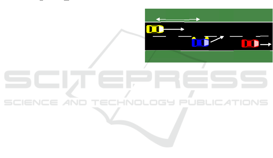
3.1 Simulation Scenario

In this contribution, a scenario on a straight road with

two lanes is considered. In total, three different

vehicles are part of the situation: On one lane, there is

the ego vehicle that is approaching a slower car,

called front vehicle. On the neighbouring lane drives

a faster car, called back vehicle. The scenario is

illustrated in Figure 3.

Figure 3: Simulated traffic scenario.

The ego vehicle is equipped with an adaptive

cruise control (ACC). Monitoring the distance to the

ahead driving front vehicle, by default the ACC

secures a safe distance by applying the brake if

getting to close. In this work, a lane change shall be

performed instead. Therefore, the viability of a lane

change manoeuvre has to be checked, which is

constrained by the approaching back vehicle.

Using suitable sensors, the ego vehicle’s ACC has

knowledge of the velocity of each vehicle, 𝑣



, 𝑣



and 𝑣



, as well as of the distances 𝑑



and 𝑑



the other cars.

3.2 Simulation Framework

The simulation framework used in this contribution

consists of a co-simulation between

MATLAB/Simulink and the microscopic traffic

simulation software Eclipse SUMO (Alvarez Lopez

et al., 2018).

Internally, SUMO uses a point mass model to

simulate the vehicles behaviour. In this framework,

the front and back vehicle are modelled with this

simple vehicle model. Both vehicles are only driving

in longitudinal direction, hence the point mass model

is suitable for the simulation. While the front vehicle

is driving at constant speed, the back vehicle may

Ego vehicle Back vehicle Front vehicle

𝑑



𝑣



𝑣



𝑣



𝑑



SIMULTECH 2022 - 12th International Conference on Simulation and Modeling Methodologies, Technologies and Applications

134

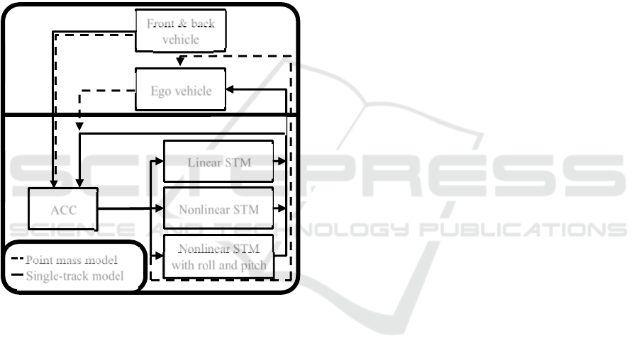
brake to avoid a crash with the lane changing ego

vehicle. This braking reaction is modelled by

SUMO’s default driver model after (Krauß, 1998).

The ego vehicle is the subject of the vehicle model

investigation, as such it is modelled by the four

already introduced vehicle models, namely the point

mass model, the linear and the two nonlinear single-

track models. The computation of the point mass

model is also performed in SUMO. As the ego vehicle

has to carry out a lane change manoeuvre, the lateral

dynamics have to be considered as well. By default,

SUMO does not model lateral movement, instead the

cars jump from lane to lane in simulation. Activating

the Sublane Model, the lateral movement is modelled

by the point mass model as well. (Semrau &

Erdmann, 2016)

Figure 4: Structure of simulation framework with point

mass model and single-track models (STMs).

The other three advanced vehicle models are

implemented in MATLAB/Simulink. These models

require the input of the steering angle, the nonlinear

single-track models need the throttle and brake pedal

positions as well. The latter inputs are computed

using a PID controller, that controls the ego vehicle’s

velocity to be constant. For the two simpler vehicle

models, this assumption of constant velocity is

required.

The steering angle is computed using a lateral

guidance model after (Fiala, 2006). This model

assumes that the driver aligns the vehicle’s driving

direction to a targeted viewpoint, in case of a lane

change this viewpoint lays on the adjacent lane. Using

a PD controller computing the steering angle, the

vehicle’s direction is adjusted.

The ACC as well is modelled in Simulink,

monitoring the distance to the front vehicle and

giving the signal that a reaction, either a lane change

or a braking manoeuvre, is necessary.

The communication between both simulations is

built using TraCI, an interface integrated in SUMO.

Using TraCI4Matlab by (Wegener et al., 2008), the

interface can be accessed from MATLAB and, with

some adaptions, also from Simulink. The co-

simulation is managed by Simulink, controlling the

simulation steps inside SUMO and recording the

necessary data for later analysis. In Figure 4, the

framework is depicted.

3.3 Data Generation

The simulation parameters 𝒙 being changed are the

velocities of the vehicles as well as the distance of the

back vehicle when the ACC signal is invoked:

𝒙𝑣



,𝑣



,𝑣



,𝑑







(8)

When performing a lane change, the viability of

the manoeuvre is evaluated regarding dangerous

interferences with the other traffic participants.

Therefore, minimum distances between the cars have

to be maintained.

Further aspects being considered are the

deceleration of the back vehicle and the lateral

acceleration and jerk the ego vehicle is exposed to

during the lane change.

The limit for the deceleration of the back vehicle

is set to a maximum of 3 m/s² according to the

recommendation by the Institute of Transportation

Engineers (ITE Technical Committee, 1989). The

limitations to the lateral dynamics conform to the

requirements specified for partially automated lane

change systems in ISO 21202 (ISO, 2020).

4 MODEL BOUNDARIES

DETERMINATION

This section presents the proposed method to choose

the simulation model with the lowest required model

by estimating their application boundaries. Therefore,

the method is described using two different machine

learning algorithms, namely SVMs and ANNs.

Afterwards, the results are evaluated and compared.

Finally, a more precise adaption to the method is

presented.

Ego vehicle

Linear STM

SUMO

Simulink

Nonlinear STM

with roll and pitch

ACC

position

lane

change

Front & back

vehicle

position

Point mass model

Single-track model

Generating a Multi-ﬁdelity Simulation Model Estimating the Models’ Applicability with Machine Learning Algorithms

135

Table 1: Parameters varied in simulation.

Parameter

Minimum

value

Maximum

value

Step size

𝑣



30 km/h 70 km/h 5 km/h

𝑣



25 km/h 65 km/h 10 km/h

𝑣



40 km/h 140 km/h 10 km/h

𝑑



50 m 200 m 25 m

To demonstrate the method, a data set consisting

of 1,505 simulation parameter combinations is

generated. The different parameters chosen for those

runs are given in Table 1. Thereby, only reasonable

combinations are considered and disregarding, for

example, combinations where the front vehicle is

faster than the ego vehicle and thus no overtaking

takes place.

Each simulation run is computed with all four

vehicle models being applied once. The lane change

is performed in each simulation run and the feasibility

of the manoeuvre is evaluated afterwards. In total, per

vehicle model 𝑀1,505 labelled data points

𝒙



,𝑦





 are available, where the label describes the

feasibility ( 𝑦





1 respectively the infeasibility

𝑦





0 of the lane change.

4.1 Data Preparation

Required is the definition of ground truth data, i.e. the

results the simulation models should produce. In

general, the best option is to choose real-world data.

As such data often is not available, like in this

contribution, the simulation model with the highest

fidelity and thus the closest real-world modelling

capability should be chosen to represent the ground

truth. Hence, in the following, the ground truth data

will be referencing the data produced with the

nonlinear single-track model with linear roll and pitch

modelling.

The next step is to evaluate the simulation models’

feasibility on given data points, i.e. the 1,505

simulation runs. By comparison of the simulation

results against the ground truth data, the models will be

determined to have sufficient fidelity if the simulation

result match the ground truth, else to be not suitable for

application. This comparison is performed for each

data point contained in the data set.

This way, a set of discrete points 𝒙



,𝑦





,

𝑚  1…1,505, is generated for each vehicle

model. These points consist of the simulation

parameters 𝒙



, at which the computed results are

compared against the ground truth, and the label 𝑦





defining the suitability of the model for this

simulation run.

Based on these discrete points, machine learning

algorithms are trained to estimate the simulation

models’ application boundaries, thus interpolating

between the given data. As a consequence, the given

data distribution should cover the simulation

parameter space sufficiently.

4.2 Classifier Training

In the following, ANNs and SVMs are trained using

the data points 𝒙



,𝑦





. As the SVM is only a

binary classifier, thus can only distinguish between

two classes, the ANNs are as well implemented as

binary classifiers for better comparison. Therefore,

for each vehicle model there will be a separate SVM

or ANN estimating if the model’s fidelity is sufficient

for a given data point. By cascading the binary

classifiers based on increasing simulation model

fidelity, the lowest fidelity model which is applicable

can be determined.

With both presented machine learning algorithms,

the data pre-processing is the same: The inputs 𝒙



are standardized to zero mean and unit variance.

Furthermore, the data set is split into two parts. 30 %

of the data is used as test data to verify the algorithms

after training. The remaining data is used for a grid

search hyperparameter optimisation in the training

process, performing a stratified 5-fold cross-

validation.

The evaluation of the trained algorithms is

performed using two metrics. Besides the standard

accuracy metric, the precision metric is used as well.

Table 2: SVMs hyperparameter variations.

Kernel Regularisation 𝐶

Kernel parameters

(Not feasible)-class

weighting

𝑟 𝛾 d

Linear 2





,…,2



- - - 1,5,10,30,50

Polynomial 2





,…,2



0,1,10 2





,…,2



2,5 1,5,10,30,50

RBF 2





,…,2



- 2





,…,2



- 1,5,10,30,50

Sigmoid 2





,…,2



0,1,10 2





,…,2



- 1,5, 10,30,50

SIMULTECH 2022 - 12th International Conference on Simulation and Modeling Methodologies, Technologies and Applications

136

The precision is defined as follows, with 𝑡𝑝

standing for true positives and fp for false positives:

Precision

𝑡𝑝

𝑡𝑝 

𝑓

𝑝

(9)

Hence, the precision is a measure for the correctness

of positive classifications. In this work, positive

classification means that the model is viable for the

given simulation parameters. Since it is desired to not

use a simulation model when its fidelity is not high

enough to produce the right results, no false positive

classifications should be made. Thus, the precision

should be 100 %. This is the constraint for all trained

classifiers to be satisfied, the accuracy metric is then

used to rank the classifiers with full precision.

4.2.1 Support Vector Machine

In the training of the SVMs, the hyperparameter

optimisation is done with respect to the kernel

functions and their respective parameters, the

regularisation and the class weighting. In terms of

kernel functions, linear, 2

and 5

degree

polynomial, gaussian (radial basis function, RBF) and

sigmoid kernels are investigated. In total, 5,670

combinations were evaluated per vehicle model, the

hyperparameters evaluated are given in Table 2.

The class weighting is chosen as additional

hyperparameter, because depending on the used

vehicle model only a small part of the data set is

assigned the class “not feasible”. To counteract the

uneven class distribution, the weight of those samples

has to be increased.

The best found hyperparameters for the vehicle

models are shown in Table 3.

Table 3: Best found SVM hyperparameter combinations.

Vehicle

model

SVM parameters

Test

accuracy

Point mass

RBF kernel, 𝐶8,𝛾2



5-times weighting

0.8894

Linear

single-track

Polynomial kernel, d= 2, 𝐶

512, 𝛾2



,𝑟 1 50-times

weighting

0.6018

The nonlinear single-track model without roll and

pitch model is not included in the table. This is

because of the similarity to the ground truth, that is in

fact only the extension by the roll and pitch

behaviour. Since the dynamics in the manoeuvre are

not remarkably high, the impact of this extension is

almost negligible – only for one data point in the

whole data set the simulation outcome differed. With

only one data point in the data set being assigned the

“not feasible” class, training a data driven model is

pointless. Hence, the standard nonlinear single-track

model will be excluded in the further evaluations of

the machine learning algorithms. In application

phase, the single data point this model is not suitable

will be computed by the ground truth model.

The two given SVM hyperparameter

combinations for the point mass model and the linear

single-track model satisfy the 100 % precision

constraint in training and validation, and achieve the

overall highest validation accuracy in training phase.

Evaluating the fully trained SVMs on the so far

unseen test data yields a precision of 100 % as well

and the accuracy given in the table. Remarkable is the

much lower accuracy achieved for the linear single-

track model, which is presumably the cost for the

precision constraint, leading to a high required class

weighting and the tendency to underestimate the

viability of the vehicle model.

4.2.2 Artificial Neural Network

For the trained ANNs, the investigated

hyperparameters are given in Table 4 with a total of

2,304 combinations evaluated.

Table 4: Hyperparameters used in ANN training.

aramete

Values

Hidden neurons







100





50,50





100,100



50,20,100,20

Activation function Sigmoid, Tanh, ELU

Dropout rate

0,0.2

L2-regularisation

0,0.01

Learning rate



,10



,10



,10



Learning rate deca

0, 0.3

(Not feasible)-class

wei

hts

1,5,10,50

Investigated are ANNs with one and two hidden

layers and varying neuron count per layer. For the

hidden layers, different activation functions are

evaluated. Furthermore, the influence of the learning

rate is considered by investigation of different start

learning rates and an optional learning rate decay of

30 % every 25 training epochs. Additionally, the

usage of regularisations methods, namely dropout and

L2-regularisation, is covered in the hyperparameter

optimisation.

The output layer of the ANNs consist of one

neuron with the Sigmoid activation function, thus the

ANNs are producing one single output ranging from

0 to 1 that can be interpreted as the “feasible” class

membership probability for the vehicle model. The

output layer is not subject to the hyperparameter

optimisation.

Generating a Multi-ﬁdelity Simulation Model Estimating the Models’ Applicability with Machine Learning Algorithms

137

During this optimisation, the ANNs are trained

for a total of 100 training epochs. Based on precision

and accuracy in the cross-validation, the best found

models are given in Table 5.

Table 5: Best found ANN hyperparameter combinations.

Vehicle

model

Hyperparameters

Point mass

Hidden neurons: 100,20

Activation function: ELU

No dropout

L2-regularisation: 0.01

Learning rate: 0.01 and 30% decay rate

Class weight: 10

Linear

single-track

Hidden neurons: 50,50

Activation function: ELU

No dropout

L2-regularisation: 0.01

Learning rate: 0.001 without decay rate

Class weight: 50

In Table 6, the performance of the two trained

ANNs on the test data is given. Important to mention

is, that none of the investigated ANNs satisfy the full

precision constraint during the hyperparameter

optimisation regarding the linear single-track model.

Even using a 100-times weighting for the “not

feasible” class resulted in only one parameter

combination fulfilling the constraint while only

achieving an accuracy of 0.08. With this restriction in

mind, a hyperparameter combination was chosen that

produced one false positive classification in the

training phase.

Table 6: Test evaluation of trained ANNs.

Vehicle model Test precision Test accuracy

Point mass 1.0 0.8341

Linear single-

track

0.9972 0.8230

4.3 Classifier Validation

For validation purposes, a larger data set is generated

in simulation. Therefore, the vehicle model for each

simulation run is chosen by the trained ANNs

respectively SVMs. In total, the new data set consists

of 5,447 data points all located in the parameter

boundaries given in Table 1 but distributed with a

finer grid. For comparison against the ground truth,

the chosen simulation runs are performed with the

nonlinear single-track model with roll and pitch

model as well.

In the following, the accuracy of the data sets

generated with the model assignment by the machine

learning algorithms as well as the computing time

required for the simulation is discussed. In Figure 5,

the computations times are visualized, in Figure 6 the

number of wrongly assigned vehicle models. Therein,

the SVMs performance is labelled with “default

SVMs”.

4.3.1 Support Vector Machine

Using the trained SVMs to assign the vehicle model

for the simulation runs, 8 of the 5,447 simulation

results differ from the ground truth data. Hence, in

0.147 % of the simulations a vehicle model is chosen

whose model fidelity is not sufficient to compute the

manoeuvre.

Mentioned should be that one of the faulty vehicle

model assignments is not made by an SVM. Both

SVMs, the one for the point mass model as well as the

one for the linear single-track model, classified their

models to be not feasible for the given simulation

parametrisation. But as already stated, the difference

in the smaller first generated data set between the

nonlinear single-track models is vanishing and thus,

no algorithm could be trained for this vehicle model.

Rather, the only known simulation parameters the

default nonlinear single-track model is not feasible

are assigned to the ground truth model manually. In

the new larger data set, another simulation

parametrisation the ground truth model should be

used is contained resulting into one wrong

assignment.

Regarding the computation times needed for the

simulation runs, with the help of the SVMs a

reduction of about 72 % is achieved.

4.3.2 Artificial Neural Network

Considering the trained ANNs for the vehicle model

assignment, a total of 29 simulation runs result in a

differing simulation outcome compared to the ground

truth. This corresponds to a wrong model assignment

in 0.532 % of simulation runs. Again, one of the

wrong model assignments is made because of the

vanishing difference between both nonlinear single-

track models.

While achieving a reduced accuracy compared to

the SVMs, the computation time reduction is

enhanced, reducing the required time by 79 %.

SIMULTECH 2022 - 12th International Conference on Simulation and Modeling Methodologies, Technologies and Applications

138

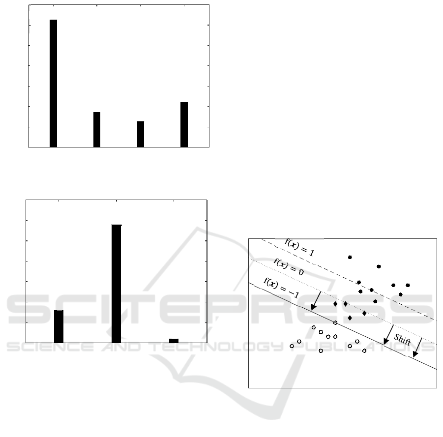
Figure 5: Computation times for data set generation.

Figure 6: Wrong model assignments in data set generation.

4.4 Shifted Classifier

As shown in the validation of the classifiers, for some

simulation runs the wrong vehicle model is chosen.

Thus, the wrong classifications are analysed

regarding the computed probabilities of class

membership.

In case of the ANNs, the output f



𝒙 ranges

from 0 to 1 and the decision boundary between both

classes is located in the middle, hence at f





𝒙





0.5. Investigating the wrong classifications, the

output was in average 0.4 away from the decision

boundary. Considering that the maximum distance is

0.5, those wrong classifications are made with a very

high probability.

For SVMs, the decision boundary is located at





𝒙



 0 and the margin spans the area of



𝒙

1 in which preferably no classification is

placed. As stated in section 2.3, small violations of

the margin are allowed in the training controlled via

the regularisation parameter.

Taking a look at the SVMs’ outputs on the wrong

classified simulation runs, the average distance from

decision boundary is at 0.276 while no distance is

larger than 0.512 and thus every data point is located

in the middle of the margin. The approach of

maximizing the margin between the classes and

having it unpopulated by data points in training

improves the robustness of SVMs on new data points

which may lay outside the training data clusters.

By shifting the decision boundary from the middle

of the margin to its boundary, the precision of the

SVM can be improved. This way, for every data point

located inside the margin the simulation model is

classified to be not feasible. Hence, for every data

point the classifiers prediction is given with an

uncertainty, the simulation model is not chosen in

favour of the precision. In Figure 7, the decision

boundary shift is visualized

Figure 7: Shifted decision boundary.

To validate this proposed approach, a third full

data set is generated in the simulation using the SVMs

already trained but shifting their decision boundaries

accordingly. The results from comparison against the

ground truth data are also shown in Figure 5 and

Figure 6.

Using the shifted SVMs indeed improved the

precision of the classifier. Now in only 1 out of the

5,447 simulation runs a wrong vehicle model is

assigned, which again is the data point not classified

because of the vanishing difference between the

nonlinear single-track models. In fact, the two shifted

SVMs achieved a precision of 100 %.

The drawback of shifting the decision boundary is

the usage of more models with higher fidelity, thus

decreasing the achievable computation time

Ground

Truth

Default

SVMs

ANNs

100

Computation time [h]

Shifted

SVMs

125.1

34.3

25.8

44.5

120

140

Default

SVMs

ANNs

Shifted

SVMs

Wrong model assignments

Variable x

Generating a Multi-ﬁdelity Simulation Model Estimating the Models’ Applicability with Machine Learning Algorithms

139

reduction. With a reduction of about 64 %, the

required time still is highly reduced.

5 APPLICATION EXAMPLE

In this final section, the generated data sets are used

to train a lane change decision system (LCDS).

Therefore, the data set generated by the shifted SVMs

and the ground truth data set are considered. The

LCDS is implemented by an SVM for each data set,

comparing the suitability of those. The goal of the

LCDS is to classify the viability of a lane change at a

given situation.

The training of the SVM is made in accordance to

Section 4.2.1, i.e. the investigated hyperparameters,

given in Table 2, are evaluated with the help of a grid

search combined with a stratified 5-fold cross-

validation. The data preparation and splitting are done

accordingly too.

Since the application is a safety relevant feature, a

lane change should not be started in unfeasible

situations. To ensure this, again the precision of the

trained classifiers is constrained to be 100 %.

Table 7: Hyperparameters and performance of trained

LCDS.

Data

set

SVM parameters

Train

accuracy

Test

accuracy

Ground

Truth

RBF kernel, 𝐶0.5,𝛾1

10-times weighting

0.9465 0.9558

Shifted

SVMs

RBF kernel, 𝐶0.5,𝛾1

10-times weighting

0.9471 0.9558

In Table 7, the in the cross-validation best

performing hyperparameter combinations are given.

The precision of both trained LCDS satisfies the full

precision constraint on both training and test data and

therefore the system is making no false positive

classifications which could result in endangering

overtaking manoeuvres. While the hyperparameters

as well as the test accuracy do not show any

differences, the training accuracy has little deviations.

Since the high similarity between both data sets is

already known, the results are not surprising.

In general, most data driven algorithms perform

well even with some noise in the training data so that

small errors in data set generation may not affect the

application. Important to mention here is that the test

data should not contain errors, thus should be taken

from the ground truth. Else, the validation of the

trained algorithms loses its significance.

6 CONCLUSION

In this contribution, a method for assigning

simulation models with different model fidelity based

on their estimated validity is proposed. Therefore, the

models’ applicability boundaries are represented by

machine learning algorithms. The algorithms

investigated are support vector machines and

artificial neural networks.

For the algorithms to learn the models’

applicability, with each considered simulation model

a small data set is generated. Comparing the

simulation results against ground truth data, the

validity of the models can be determined at discrete

simulation parametrisations. Given this data,

classifiers can be fit to estimate the simulation

models’ feasibility.

Using these classifiers, larger data sets can be

generated only using a valid simulation model with

the lowest computational effort.

It is shown, that the proposed method can be used

to highly reduce the required computation time for

simulation data generation. Using ANNs or SVMs, a

computation time reduction of 79 % resp. 72 % is

achieved while generating a wrong simulation result

in only 0.53 % resp. 0.15 % of generated data.

Furthermore, it is proposed to shift the SVM’s

decision boundary to improve the accuracy of the

generated data set. This way, no loss in data set

accuracy was produced with the drawback of a lower

computation time reduction of 64 %.

Finally, a lane change decision system is

implemented using the generated data set. It is shown,

that the developed system achieves the same accuracy

as if it was trained on the highest fidelity model only.

Overall it can be stated, that the proposed method

can greatly reduce the required computation times

when generating large data sets by simulation.

Regarding the used machine learning algorithms, the

investigated SVMs overperform the ANNs in terms

of accuracy. In cases where the data set accuracy is

crucial, it is recommended to use the proposed shifted

SVMs for the classification.

A drawback of the method is the required

preparation of an initial data set for each investigated

simulation model. This data set should cover the

simulation parameter space in a sufficient manner to

provide enough information for the model

applicability estimation. Needing only small data

sets, the time required to generate the initial data sets

may exceed the later time savings.

It is also shown, that for models with high

similarity to the ground truth the method is not

applicable. In such case, only a vanishing part of the

SIMULTECH 2022 - 12th International Conference on Simulation and Modeling Methodologies, Technologies and Applications

140

data set contains information about the simulation

model’s applicability and the training of the machine

learning algorithms will fail.

Further research will investigate the possibility to

perform the initial estimator learning in an iterative

approach starting only with a small amount of initial

data points, thus being able to reduce the preparation

effort.

REFERENCES

Alvarez Lopez, P., Behrisch, M., Bieker-Walz, L.,

Erdmann, J., Flötteröd, Y.-P., Hilbrich, R., . . . Wießner,

E. (2018). Microscopic Traffic Simulation using

SUMO. Paper presented at the The 21st IEEE

International Conference on Intelligent Transportation

Systems, Maui, USA.

Biehler, J., Gee, M. W., & Wall, W. A. (2015). Towards

efficient uncertainty quantification in complex and

large-scale biomechanical problems based on a

Bayesian multi-fidelity scheme. Biomechanics and

Modeling in Mechanobiology, 14(3), 489-513.

doi:10.1007/s10237-014-0618-0

Bishop, C. M. (2006). Pattern recognition and machine

learning: New York : Springer.

Fernandez-Godino, M. G., Park, C., Kim, N., & Haftka, R.

(2017). Review of multi-fidelity models.

Fiala, E. (2006). Mensch und Fahrzeug: Fahrzeugführung

und sanfte Technik [Human and vehicle: Vehicle

guidance and smooth technology]. Wiesbaden: Vieweg.

Gron, A. (2017). Hands-On Machine Learning with Scikit-

Learn and TensorFlow: Concepts, Tools, and

Techniques to Build Intelligent Systems: O'Reilly

Media, Inc.

Heißing, B., & Ersoy, M. (2011). Chassis Handbook:

Fundamentals, Driving Dynamics, Components,

Mechatronics, Perspectives. Wiesbaden:

Vieweg+Teubner.

ISO. (2020). Intelligent transport systems - Partially

automated lane change systems (PALS) - Functional /

operational requirements and test procedures.

ITE Technical Committee. (1989). Determining Vehicle

Change Intervals: A Proposed Recommended Practice.

ITE Journal, 57, 27-32.

Krauß, S. (1998). Microscopic Modeling of Traffic Flow:

Investigation of Collision Free Vehicle Dynamics.

Retrieved from

Pacejka, H. B. (2012). Tire and Vehicle Dynamics (Third

Edition). Oxford: Butterworth-Heinemann.

Paulweber, M. (2017). Validation of Highly Automated

Safe and Secure Systems. In D. Watzenig & M. Horn

(Eds.), Automated Driving: Safer and More Efficient

Future Driving (pp. 437-450). Cham: Springer

International Publishing.

Schölkopf, B., & Smola, A. J. (2018). Learning with

Kernels: Support Vector Machines, Regularization,

Optimization, and Beyond: The MIT Press.

Schramm, D., Hiller, M., & Bardini, R. (2018). Vehicle

Dynamics - Modeling and Simulation: Springer-Verlag

Berlin Heidelberg.

Semrau, M., & Erdmann, J. (2016). Simulation framework

for testing ADAS in Chinese traffic situations. Paper

presented at the SUMO2016, Berlin.

Sieberg, P., Blume, S., Reicherts, S., & Schramm, D.

(2019). Nichtlineare modellbasierte pradiktive

Regelung der Fahrzeugdynamik in Bezug auf eine

aktive Wankstabilisierung und eine Nickreduzierung.

[Non-linear model-based predictive control of vehicle

dynamics in terms of active roll stabilization and pitch

reduction]. Forschung im Ingenieurwesen, 83(2), 119-

127. doi:10.1007/s10010-019-00337-6

Sovani, S., Johnson, L., & Duysens, J. (2017).

Incorporating high fidelity physics into ADAS and

autonomous vehicles simulation, Wiesbaden.

Wegener, A., Piórkowski, M., Raya, M., Hellbrück, H.,

Fischer, S., & Hubaux, J.-P. (2008).

TraCI: an interface

for coupling road traffic and network simulators. Paper

presented at the Proceedings of the 11th

communications and networking simulation

symposium, Ottawa, Canada.

Generating a Multi-ﬁdelity Simulation Model Estimating the Models’ Applicability with Machine Learning Algorithms

141