Multi-factor Prediction and Parameters Identification based on
Choquet Integral: Smart Farming Application
Yann Pollet
1a
, Jérôme Dantan
2b
and Hajer Baazaoui
3c
1
CEDRIC EA 4629, Cnam, Paris, France
2
Interact UP 2018.C102, Institut Polytechnique UniLaSalle, Mont-Saint-Aignan, France
3
ETIS UMR 8051, CY University, ENSEA, CNRS, Cergy, France
Keywords: Choquet Integral, Decision Model, Parameter Identification, Smart Farming.
Abstract: In this paper, we consider the domain of smart farming aiming at agronomic processes optimization, and,
more particularly, the issue of predicting the growth stages transitions of a plant. As existing automated
predictions are not accurate nor reliable enough to be used in the farming process, we propose here an
approach based on Choquet integral, enabling the passage from multiple imperfect predictions to a more
accurate and reliable one, considering the relevance of each source in the prediction as well as the interactions,
synergies, or redundancies between factors. Identifying the parameter values defining a Choquet-based
decision model being not straightforward, we propose an approach based on an observation history. Our
proposal defines an evaluation function assigning to any potential solution a predictive capability, quantifying
a degree of order present in its output, and an associated optimisation process based on truth degrees regarding
a set of inequalities. A case study concerns smart farming, the prototype we implemented enabling, for a given
culture and several input sources, to help farmers to predict the next growth stage. The experimental results
are very encouraging, the predicted day remaining stable despite presence of noise on evidence values.
1 INTRODUCTION
Decision-based applications and environments all
require an intelligent combining of data coming from
multiple sources, including sensors, humans, and
algorithms. Combining data with relevant
aggregation operators and identifying parameters
corresponding to the best decision model is a
challenging issue, due, among those, to the amount of
available data to be considered. Several aggregation
operators have been adapted to be used in a variety of
information fusion problems, the choice of an
aggregation operator depending essentially on the
nature of available information as well as the types of
values to be used: quantitative, qualitative, binary, ….
We consider here the agricultural domain, a
strategic area where, today, a major issue consists in
increasing field productivity while respecting the
natural environment and farms sustainability,
requiring the development of advanced decision
a
https://orcid.org/0000-0002-5819-355X
b
https://orcid.org/0000-0001-7007-8725
c
https://orcid.org/0000-0002-1224-1002
support tools. In this context, a key issue in
maximizing crop efficiency remains this of making
reliable predictions regarding growth stage transition
of plants, especially dates of transitions from the
current stage to the next one. Such a prediction should
be based on various available sources of information,
that deliver in practice more or less accurate and
reliable information. It will enable the farmer to
prepare and perform relevant actions at the best
instant with a maximized efficiency.
In this context, multi-factor decision requires use
of aggregation functions, such as fuzzy integrals,
more precisely the well-known integral of Choquet.
This latter is defined from a fuzzy measure and allows
to consider the possible interactions between factors
(Sugeno, 1974). Choquet integral will be used here as
an operator of aggregation, in charge of fusing
multiple imperfect predictions into a more certain and
accurate one, exploiting source diversity to get a more
significant and reliable information for guiding
decisions.
340
Pollet, Y., Dantan, J. and Baazaoui, H.
Multi-factor Prediction and Parameters Identification based on Choquet Integral: Smart Farming Application.
DOI: 10.5220/0011317900003266
In Proceedings of the 17th International Conference on Software Technologies (ICSOFT 2022), pages 340-348
ISBN: 978-989-758-588-3; ISSN: 2184-2833
Copyright
c
 2022 by SCITEPRESS – Science and Technology Publications, Lda. All rights reserved

In this paper, we focus on the Choquet integral,
proposing a parametric function for data aggregation.
We put our interest on an application of smart
farming, proposing a way to identify the parameters
of a growth stage prediction model. We point out that
in a previous work (Dantan, 2020), we proposed a
fuzzy decision support environment for smart
farming ensuring better data structuration extracted
from farms, and automated calculations, reducing the
risk of missing operations.
Our aim here is to identify the parameters of a
Choquet-based prediction using a training dataset
including past data delivered by sources jointed to
observed evidence, proposing parameter values based
on observed preferences. Our proposal defines 1) an
evaluation function enabling to quantify the
prediction capability of any potential solution, based
on truth degrees of inequalities issued from evidence,
2) on algorithm adapted from the classical gradient
descent providing a robust solution. The originality of
our proposal relies on one hand to identify the
parameters only using inequalities, without values of
the function to be learnt, and, on the other hand, to
robustness of the obtained solution due to its least
specificity related to training data.
Our operator, based on Choquet integral, should
apply ponderations to each information source,
considering possible interactions, synergy
complementarity, or, conversely, partial redundancy,
between them. It will transform the input fuzzy sets
delivered to sources into a new fuzzy set aggregating
the input sources and delivering a global value of
confidence based on several source-dependent inputs.
The solution to our problem will be the optimum of
our evaluation function, the obtained evaluation value
quantifying both the ability of the solution to make
right predictions and the robustness of this solution.
The remainder of this paper is organized as
follows. Section 2 presents the preliminaries and the
related works. Then, in sections 3, 4 and 5, we
formalize the problem and detail our proposal and its
main components including the proposed algorithm.
Section 6 is dedicated to a presentation of the
numerical results and the interpretation of the
obtained results. Finally, we conclude and present our
future work in section 7.
2 STATE OF THE ART AND
MOTIVATIONS
In this section, we first present preliminaries, and then
an overview of the related research concerning
Choquet integral and decision models along with our
motivations and objectives.
2.1 The Smart Farming Application
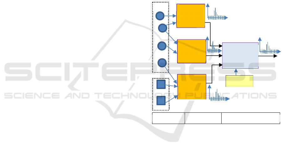
The overall functional architecture of our prediction
process is presented on the figure 1. We have three
levels:
 Sensor and data acquisition level, that includes
terrain sensors, aircraft and sattelite images
acquisition, and external data collection
through Web Service invokations;
 The level of prediction sources, including the
various algorithms in charge of performing
exprimental or more complex predictions;
 The global aggregation level.
Figure 1: Functional schema of growth stage predictions.
2.2 The Choquet Integral
Choquet integral has been adopted taking into
account the minimal set of hypothesis required on the
nature of data, as well as its ability to properly model
multiple interactions between sources, including
partial redundancy and possible substituability of
them. In addition, we must mention the simplicity of
calculation to be perfomed at real time, and the
human understandability of the various model
parameters.
The notion of fuzzy integral, based on the concept
of fuzzy measure (Sugeno, 1974), also called
capacity, enables to assign a relative importance, not
only to each individual decision criterion, but also to
any subset of criteria. In the context of multi-criteria
analysis, the weight or importance of the set of
Aggregation
operator
Source-
specific
predictor
Source-
specific
predictor
Source-
specific
predictor
Aggregated
prediction
Sensors
Other sources
Single source
predictions
Measures
Data
Training
Sensor level Source level Aggregation
Multi-factor Prediction and Parameters Identification based on Choquet Integral: Smart Farming Application
341

criteria association influences the entire combination
of criteria, which could be also defined.
Considering a capacity μ on the set N = {1, …,
n}, i.e. a function from 2
N
into IR
+
such as μ(Ø) = 0,
μ(N) = 1, and monotonic (i.e. S, T ⊆ N then μ(S) ≤
μ(T)), the discrete Choquet integral related to the
capacity μ is defined as the function that associates to
any n-uple x = (x
1
, …, x
n
) ∈ IR
n
.
C
μ
(x
1
, …, x
n
) := 
i-1
i=n
(μ(A
σ
(i)
) - μ(A
σ
(i+1))
).x
σ
(i)
(1)
Where σ is a permutation on N such as x
σ
(i)
≤ ….
≤ x
σ
(n)
, and where:
A
σ
(i)
:= {σ(i), …, σ(n)} ∀ i ϵ N, A
σ
(n+1)
= Ø (2)
To simplify notations, we shall write, for any
subset {i
1
, …, i
p
} of N:
μ({i
1
, …, i
p
}) = μ
i1, …, ip
(3)
A particular case of Choquet integral is the simple
weighted sum 
i
a
i
.x
i
(
i
a
i
= 1), the values μ(S), S
⊆ N, generalizing here a classical weight vector.
Limit cases of Choquet integral are the Min and Max
operators.
The Choquet integral enables the representation of
non-additive criteria, i.e., with interactions between
pairs or groups of criteria. Its interest consists mainly
in identifying, during a decision-making process,
given a set of values that meet this situation, the better
quality alternative.
2.3 Related Works
The Choquet integral is based on two fundamental
concepts: utility and capacity.
A utility function aims to model the preferences
of the decision maker regarding various possible
input values x
i
. Utility functions can be seen as
making it possible to translate the values of the
attributes x
i
into a satisfaction degree (Kojadinovic,
2009). Utility values are commensurable, monotonic,
and ascending because, if an alternative a is preferred
to b, then u (a) ≥ u (b) (Labreuche, 2009).
A capacity models the fuzzy measure on which
the integral is based and summarizes the importance
of the criteria by aggregating utility functions,
generalizing traditionally used weight vector. The
learning ability of the Choquet integral has been
demonstrated, mainly in (Grabisch, 2008). Functions
dealing with data mining issues such as least square
and linear programming have been used in this
context. Preference learning consists in observing and
learning the preferences of an individual, precisely in
particular when ordering a set of alternatives, to
predict automatic scheduling of a new set of
alternatives (Fürnkranz, 2012).
The Choquet integral learning function is based
on a set of concepts that make it possible to leverage
the consideration of user preferences (or decisions)
and the interaction and/or synergy between the
various criteria for data aggregation. Given a
preferential ordering on a sample learning, the
discrete Choquet integral is able to quantify, then
learn, the relative weights of the different quality
metrics.
In the literature, fuzzy integrals have been used
for different purposes, for preferences or opinions
fusion from a variety of sources, and several
applications and extensions of fuzzy integrals have
been developed. In (Vitor de Campos Souza, 2018),
the authors have proven that the use of fuzzy neural
network is more effective than the decision tree
algorithms often used in the literature. The fuzzy
neural network model allows precision improvement
and less redundancy in decision-making.
In our previous work, we have proven that
applying Choquet integral to order data sources
according to the user's preferences, is an interesting
and challenging area of research and can lead to more
relevant results (Dantan, 2020). One originality of the
work described in this paper consists in the proposal
of an evaluation function attaching to any potential
solution a degree of acceptability, based on truth
degrees of inequality.
3 PROBLEM STATEMENT
Considering a crop with n prediction sources,
information delivered by a source will consists in a
sequence of confidence levels x
i
(d) ∈ [0,1] associated
to future days 1, …, D, given a temporal horizon of D
days. x
i
(d) value reflects the belief of the i
th
source
regarding the occurrence of transition at d day, from
the present phenological stage to the next one. We
have so as many functions d ∈ {1, …, D} → x
i
(d) ∈
[0, 1] as prediction sources i=1, …, n, and x
i
(d) can
be seen as the membership function of a fuzzy subset
of {1, …, D}, 0 meaning a null confidence, and 1 the
maximum value, as presented on figure 2.
No hypothesis can be made here on confidence
levels semantics. In particular, these levels are not
probabilities, only inequalities between two values
issued from the same source being significant. Note
the case with several days having all a 1 value is
possible, reflecting inaccuracy of the prediction.
ICSOFT 2022 - 17th International Conference on Software Technologies
342

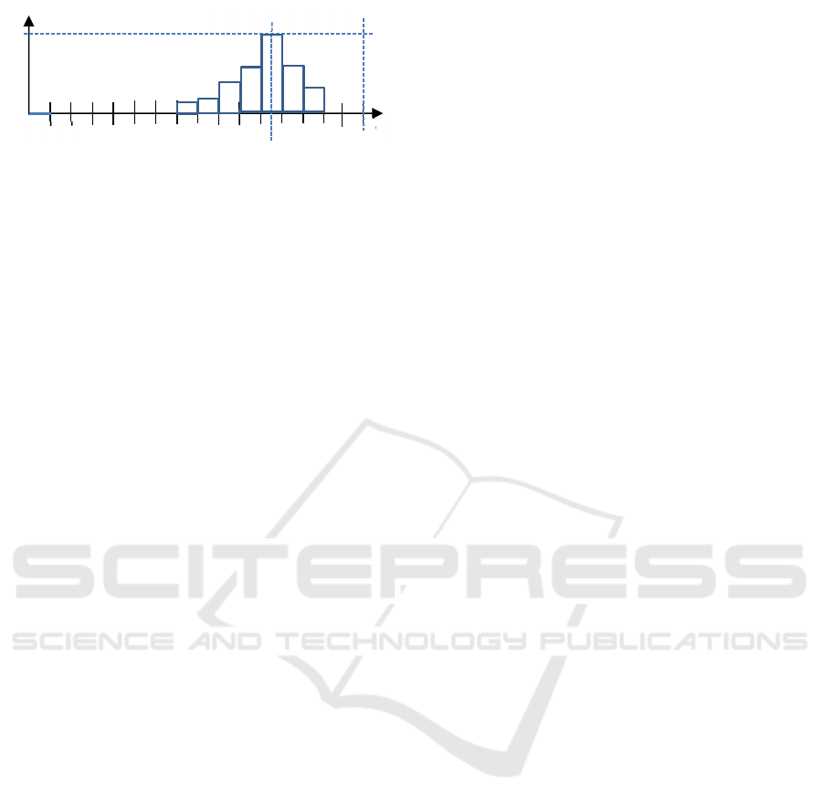
Figure 2: Fuzzy prediction on a temporal horizon of D days.
We use the Choquet integral as an operator of
aggregation, in charge of fusing the later n fuzzy
predictions into a more certain and accurate one. It is
expected from source diversity more significant and
reliable information for guiding decision. This
operator will have to apply proper ponderations to
each information source, considering possible
interactions, synergies complementarities, or, at
contrary, partial redundancies, between them. It will
transform n fuzzy subsets into a result fuzzy subset,
aggregating the n input sources. Our goal is to enable
an automated estimation of Choquet integral
coefficients based on a recorded history, i.e., on a
dataset of past source predictions, in addition to the
corresponding observed evidence.
X = (x
1
, …, x
n
) denoting a confidence vector, n
being the number of sources, the training dataset
consists in P sessions regarding the same plant, a
session being related to a field at a given period. For
each session, we have a sequence of X
d
, prediction
vectors for days d=1, …,D, in addition to d
Tr
, the real
day of transition, a posteriori observed for this
session.
Available information may be expressed thanks to
a set of R = (D-1).P inequalities :
C
μ
(X
k
) < C
μ
(X
evidence(k)
) (4)
with k, evidence(k)
∈ [1, D.P], evidence(k) (≠ k)
being the d
Tr
transition day for the session containing
the day k.
Our problem is to learn a μ capacity, i.e. the values
of the 2
n
– 1 parameters μ
i
, μ
i,j
, μ
i,j,k
, … satisfying the
above inequalities. Despite some of these may be
trivially satisfied by any Choquet integral, i.e., for any
μ, we keep them as input data of our problem,
intensities of differences being considered here as
significant pieces of information. It is the same for
inequalities implicitly satisfied by transitivity, e.g.
C
μ
(X) < C
μ
(Z), if X < Y and C
μ
(Y) < C
μ
(Z).
Based on Choquet integral definition, available
information may be expressed under the form of R
inequalities, applying on linear expressions:
a
k
1
.
μ
1
+…+ a
k
n
.
μ
n
+ a
k
1
,1
.
μ
1,2
+ …+ a
k
n-1,n
.
μ
n-1,n
+
….. + a
k
1,
…
,n
.μ
1,
…
,n
> 0 , k=1, …,R
(5)
That is, using a matrix notation:
[A]
k
.[μ] > 0, k=1, …, R (6)
where [A]
k
is the (2
n
-1) row vector [a
k
1
, ..., a
k
n
,
a
k
1,1
, …, a
k
n-1,n
, ….. , a
k
1,
…
,n
] and [μ] the (2
n
-1)
column vector [μ
1
, ..., μ
n
, μ
1,1
, …., μ
n-1,n
, … , μ
1,
…
,n
]
That we may denote:
[A].[μ] > 0 (7)
[A] being the rectangular matrix build with rows
[A]
k.
, and coefficients μ
i
, μ
i, j
, μ
i, j, k
, etc., satisfying
the minimal set of constraints:
μ
i
≤ μ
i,j
,∀i, j, i≠j,
μ
i,j
≤ μ
i,j,k
, ∀i, j, k, i≠j, j≠k, k≠i, ….
With μ
i
≥ 0 ∀i, and μ
1, …,n
≤ 1 (8)
that may be more concisely expressed by:
μ(S) ≤ μ(S’) ; |S’| = |S| + 1, S ⊂ S’
with μ(Ø) = 0 and μ
1, …,n =
μ(2
N
) ≤ 1 (9)
We have here no values regarding a function to be
learnt, but only a set of statements regarding
inequalities. So, a direct identification method is not
applicable. For building the solution, we are
expecting here 1) a scalable algorithm, i.e., an
algorithm that will be efficient for a huge training
dataset with a time of execution linearly increasing
with respect to the number of sessions P. In addition,
2) we consider data as potentially inaccurate, the
solution having to be robust in case of conflicting
examples, i.e., the expected solution should be able to
tolerate some local “nearly satisfied” inequalities. At
last, 3) we are expecting a solution easily improvable
by increments when new data are acquired.
4 THE PROPOSED APPROACH
Except in singular cases, joint inequalities (5) and (8)
have either zero or an infinity of solutions. In practice,
as numerous x
i,
provided by sources are not perfect
values, local violations of inequalities (5) should be
accepted. So, we do not consider only exacted
solutions, but all potential solutions with a μ vector
satisfying the only strict inequalities (8). On this
domain of potential solutions, we shall optimize an
evaluation function reflecting the expected
d
x
i
1
Highest belief
D
Presen
t
Multi-factor Prediction and Parameters Identification based on Choquet Integral: Smart Farming Application
343

characteristics considered above, in order to get the
optimized solution.
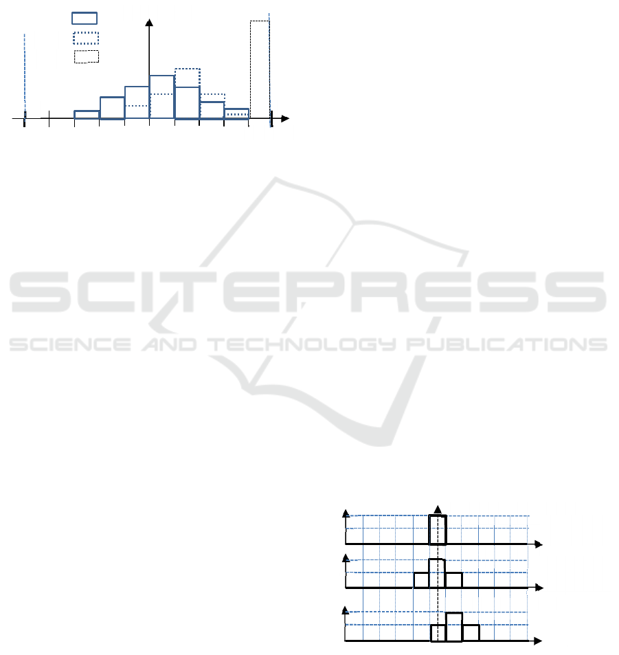
4.1 Evaluation Function
Considering a given μ capacity, the empirical
distribution of [A]
k
.[μ] values on [-1, 1] looks as the
following histogram (figure 3).
Figure 3: Empirical distribution of inequality intensities
with various [μ].
We must choose μ in such a way this distribution
has the less as possible negative values (correct
predictions), and the greatest as possible positive
values (lowest specificity). This is illustrated on
figure 3, case 2 being better than case 1, ideal case
being this where all [A]
k
.[μ] would be exactly equal
to 1.
To meet such a distribution, we choose to
minimize an additive cost function having the
following form:
Φ (μ) = 
k=1, …,R
ϕ ([A]
k
.[μ]) (10)
Where ϕ is a function : [-1, 1]
m
→ IR+ continue,
strictly decreasing, and C1 class, with:
 ϕ (1) = 0 (case of perfect ordering);
 Lim
δ →
-1
ϕ (δ) = +∞ (case of worst ordering).
ϕ being in addition strictly convex: ∀δx > 0, ϕ(-δx)
+ ϕ(δx) > 2.ϕ(0) will give us assurance that a defect
of ordering corresponding to -δx is not compensated
by an overage of same intensity δx.
So, we can choose a local cost function:
ϕ (x) = - L.log
2
(½.(x + 1)), with L ∈ IR
+
(11)
Normalizing the expression of ϕ(x) with respect
to R, number of inequality statements, we get:
Φ (μ) = -(1/R). 
k=1, …,R
log
2
(½.([A]
k
.[μ] + 1)) (12)
This quantity quantifies the average “degree of
order” present in results delivered by C
μ
integral with
respect to evidence, expressing thus the predictive
capability of C
μ
with the chosen [μ]. This order
reflects both the crispness of the aggregated
prediction and its degree of matching with reality.
More generally, we may use a function:
Φ (μ) = - (1/R). 
k=1, …,R
log
2
(ν([A]
k
.[μ]) ) (13)
ν(δ) being a fuzzy comparator, associating to any
[A]
k
.[μ] ∈ [-1, 1] a value ∈ [0,1], that is in fact the
degree of truth of the assertion:
[C
μ
(X
d
) < C
μ
(X
Evidence(d)
)] (14)
ν may be for example ν(δ) = ½.λ.(1 + erf((√2.δ)),
where erf is the Gauss error function, enabling us to
take into account a known inaccuracy of input values
x. Our first expression corresponds just to the case
where ν is the linear comparator ν(δ) = ½.(δ + 1).
4.2 A Measure of Order
More generally, one can associate to any fuzzy
prediction x
i
, i=1,…, D, a quantity S reflecting an
actual lack of information in comparison with
evidence, the considered prediction being here either
information delivered by a single particular source, or
a result from a multisource aggregation operator.
S = - (1/(D-1)). 
k=1, …, D-1
log
2
(ν([A]
k
.[μ])) (15)
We can equivalently consider a quality factor
defined by Q = 2
-
S
ϵ [0, 1], 1 being the value
corresponding to a perfect prediction, and 0 standing
for an absence of information. The figure 4 presents
some examples of different qualities of prediction.
Figure 4: Examples of fuzzy predictions with associated S
values.
Frequency
1
[A]
k
.[μ]
Case 1
Case 2
Ideal
-1
Day of transition
Prediction 1 (ideal)
S = 0
(Q = 1)
Prediction 2
Prediction 3
S = 0.08
(Q = 0.95)
S = 0.63
(Q = 0.64)
D=11
ICSOFT 2022 - 17th International Conference on Software Technologies
344

Φ(μ) appears as the average value of S on the
given training dataset. It represents the expected
value of S related to a new prediction and quantifies
thus the performance of the aggregation operator.
5 ALGORITHM
The function Φ(μ) being strictly convex as a sum of
strictly convex functions, and then, having a unique
minimum, we use a simple gradient descent method
to minimize it.
At first, we shall combine this basic method with
the use of a penalization function in order to keep
candidate solutions inside the limits of the domain of
validity defined by the set of inequations (8).
5.1 Gradient Descent
The solution is a (2
n
–1) dimension vector [μ] = [μ
1
, ...,
μ
n
, μ
1,1
, …., μ
n-1,n
, … , μ
1,
…
,n
], denoted here [m] = [m
1
,
m
2
, ….., m
2
n
-1
], minimizing Φ. Φ may be expressed
as:
Φ(m) = - L.
k=1, …,R
Log(1+ 
i=1, …,2
n
-1
a
k,i
.m
i
)
(16)
Where a
k,i
is the i
th
component of [A]
k
, and where
L=1/(R.Log(2)), the j
th
component of the gradient
being:
∂Φ/∂m
j
(m) = -L.
k=1, …,R
a
k,j
/(1+
i=1, …,2
n
-1
a
k,i
.m
i
)
(17)
First, we calculate, for each statement of
inequality k, the 2
n
-1 values a
i,k
. Then, a loop
calculates successive iterations m
p
of the m vector,
according to the formula:
m
p+1
= m
p
- ε
p
.grad(m
p
) + Ψ(m
p
) (18)
Where grad(m
p
) is the gradient vector [∂Φ/∂m
j
(m
p
)],
and where Ψ(m
p
) represents a penalization related to
domain frontiers, i.e. associated to the constraints μ
i,
≥ 0, μ
i1,i2
≥ μ
i1
, μ
i1,i2, i3
≥ μ
i1,i2
, …, and ε
p
being a step
size with an initial value ε
0
, and possibly updated at
each iteration.
The iteration loop stops when || m
p+1
– m
p
|| < η, where
η
is a predefined value.
5.2 Penalization and Projected
Gradient
We consider the frontiers of the solution domain with
the use of a penalization function m → Ψ(m) defined
as:
Ψ(m) = 
i=1, …,n
θ(μ
i
)
+ 
S
⊆
N,S
≠
Ø,S
≠
N,{i}∩S=Ø
θ(μ
S
∪
{i}
-μ
S
) (19)
where θ is continuous and derivable, θ(x) ≈ 0 for
x > 0, θ(x) being large positive for x < 0. E.g., for n =
2, to express the required constraints μ
1
≥0, μ
2
≥0,
μ
1
≤μ
1,2
, μ
2
≤μ
1,2
, and μ
1,2
≤ 1, we shall have Ψ([μ
1
, μ
2
,
μ
1,2
]) = θ(μ
1
) + θ(μ
2
) + θ(μ
1,2
- μ
1
) + θ(μ
1,2
- μ
2
) + θ(1 -
μ
1,2
).
We use here a simple exterior penalization θ(x) =
min(x, 0))
2
/(2. γ), γ being a parameter in relationship
with the expected result accuracy (e.g., η = 0.01).
As convergence process may be long, especially
when the optimum solution is on the domain frontier,
i.e. on one of the canonical hyperplanes μ
i
=0, …, μ
i1,
…, i
p
=μ
i1, …, ip, ip+1,
…, μ
i1, …, in
=1, instead of a
penalization, we use an adaptation of projected
gradient method, that is simple in our case where
domain is a convex polytope closed by a set of
canonical hyperplanes.
At each iteration, we evaluate the functions ω
i
(μ)
= μ
i
, …, ω
i1, …, ip, ip+1
(μ) = μ
i1, …, ip, ip+1
- μ
i1, …, ip
, and ω
i1,
…, i
n
(μ) = 1 - μ
i1, …, in
, a negative ω value meaning the
candidate solution vector m
p
is out of the domain. In
this case, the actual step ε
p
is chosen in such a way
that candidate solution is put just on the frontier.
Then, at the next iteration, gradient grad(m
p
) is
replaced by grad(m
p
)
proj
, orthogonal projection of
grad(m
p
) on the considered hyperplane, ensuring that
the new candidate solution will remain inside the
domain.
5.3 Overview of the Algorithm
The algorithm is shown in pseudo-code (cf. Figure 5).
The first line initializes the Choquet integral
coefficients, number of days and sources of the
current session and penalization function (pf).
Multi-factor Prediction and Parameters Identification based on Choquet Integral: Smart Farming Application
345

Figure 5: Algorithm in pseudo-code.
6 CASE STUDY AND
NUMERICAL RESULTS
The smart farming consists in the implementation of
"intelligent" tools intended to support and control all
the actions required on the crops based on collected
information. In this context, sensors attached to
agricultural plots carry out physical variables,
enabling to periodically collect and store data. All
these sources provide partial, imprecise, and
uncertain information about reality.
Therefore, in smart farmer context, at first, it is
necessary to develop an estimated future state of the
reality regarding the development of culture, based on
a set of imperfect measures. Such an estimate state
has to be maintained and improved over time. Our
evaluations of the proposed approach are led in the
context of crop monitoring, and aim at predicting the
growth stages, called phenological stages, of a plant.
So, in each stage, we propose to predict (reconsidered
and refined in real time according to the new available
information/data) the transition date to the next stage
of plant development. This is a key factor for the
farmer, which will allow each action to be carried out.
6.1 Experimental Setup
In a smart farming application, the days of transition
from a growth stage to the next one is a very
important issue for operators like farmers, who can
then take the right actions at time t, to plan the
sequence of actions to be taken with the right timing,
e.g. fertilization, watering, other treatments. The n
sources are then the predictions delivered according
to n different methods with various input data and
processes.
As an illustrative example, we base our
experiment, for a given culture, on three sources of
input, which are:
 The classical empirical calculation called
“growing degree-days method”;
 A statistical model of the plant;
 A digital image processing.
6.1.1 Classical Empirical Calculation
The growing degree-days method is based on the
cumulative daily variations of observed ambient
temperature, according to the following formula,
valid in absence of any disturbing element (e.g.
stressing environmental factors like unseasonal
drought or disease) and under given temperature
conditions:
GDD(d)=
n=D0, 1, …, d
[(T
max
(n) – T
min
(n))/2 -T
base
] (20)
Where:
 T
max
(n) and T
min
(n) are the minimum and
maximum temperature measured during day n,
computed from day D
0
, changeover day in the
current growth stage;
 T
base
is a constant value depending on the plant
(called “zero vegetation temperature”).
This calculation, based on daily measured
temperatures allows the estimation of changeover day
to the next stage (day d*) for which GDD(d*) reaches
a known value, denoted DJ0 I, specific constant
depending on both the current growth-stage and the
considered plant). The calculation will be based on
the weather data recorded up to the current day d, then
on the weather forecast from day d+1. In practice,
such a prediction is attached to low precision but quite
good trueness. In general, the closer the planned
changeover date is, the more precise is the prediction
on day d, this prediction being moreover daily
refined.
Initialize muij, d, s, epsilon, pf(x)
/* 2-dimensions confidence table for
data source/day */
list[d][s]sessionDS
/* Confidence at transition day */
list[s] transitionDS
list[d] deltaEquationList = map(-,
(CreateEquation(transistionDS),
createEquation(sessionDS)))
list[d] entropyEquationList = map(-log2
(erf(x)), deltaEquationList)
do {
dict gradientDict[key=“muij”].values
= sum (map(diff(muij),
EntropyEquationList(muij)))
dict
penalizationDict[key=“muij”].values =
sum(map(min(diff(pf(x)), muij),0)
/* Penalization */
new_muij = muij
+ epsilon* (gradientDict[“muij”]
+ penalizationDict [“muij”])
} while (sqrt(sum(new_muij-muij)**2) <
epsilon
ICSOFT 2022 - 17th International Conference on Software Technologies
346

6.1.2 Statistical Model of the Plant
The statistical model of the plant. Such a model
depends on various parameters, such as the type of
plant and the considered region. From data given as
input and representative of the context (e.g. average
temperature or soil quality indexes), such a model
provides a prediction (by the application of a formula
or an extrapolation from a table).
This prediction will be affected of a certain degree
of confidence that depends on the quality of the
model, and more or less good fits to empirical data.
In practice, a prediction will therefore result in a
confidence interval, i.e. a confidence interval
associated to a given confidence threshold.
6.1.3 Digital Image Processing
Observation by digital image processing delivers a
measurement based on visual characteristics (red and
infrared channels) of the observed plant, issued from
a satellite image, with calculation of NDVI
(Normalized Difference Vegetation Index).
Using different cameras in different locations,
such a source can also perform a digital image
processing aiming at extracting typical visual
characteristics of growth stages, e.g. specific forms
and their degree of development. The results issued
from such growth-stage prediction methods are also
imprecise.
6.2 Experimental Evaluation
The case study concerns the cultivation of winter
wheat in Normandy, which is a region with a
temperate oceanic climate in France. This case is
based on simulation data mixed with data from past
experiences. In this example, we are at the beginning
of stage 8 (maturity) and we are trying to predict the
end of ripening and therefore the beginning of stage 9
(senescence), in order to harvest wheat. The prototype
was developed in Python 3 programming language.
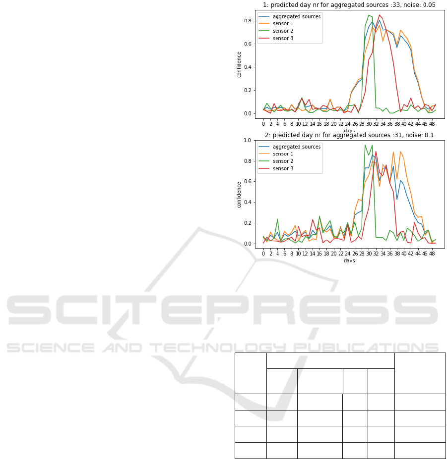
In order to assess the robustness of our algorithm,
we placed as inputs noisy sensor confidence data,
with Gaussian noises of increasing standard
deviations. Figure 6 illustrates examples of graphs
obtained with noisy data sources.
We performed a simulation with noisy input 50
times per noise value (Gaussian noise with standard
deviation from 0.05 to 0.15). For each simulation, we
computed descriptive statistics about the predicted
day of passage (cf. table 1). These analyses seem to
show a certain robustness of the algorithm, even with
Figure 6: Predicted days for the next growth stage.
noisy signal. The predicted day does not seem to vary
significantly. Table 1 contains the summary of the
simulations.
Table 1: Experimental results.
Noise
Predicted day Avg max
Choquet
integral
value
Avg
Std
deviation
Min Max
0.05 31.72 1.266 30 35 0.806
0.075 32.26 1.467 30 35 0.809
0.1 32.52 1.459 30 35 0.821
0.15 32.1 1.992 29 37 0.880
7 CONCLUSION AND FUTURE
WORK
In this paper, we proposed a Choquet-based decision
model associated to a parameter identification
approach. We explored the genericity, the non-
additivity and the synergies between the different
criteria parameters, related to the Choquet integral, to
propose a solution as an answer to the difficulty of
defining several parameters values.
Multi-factor Prediction and Parameters Identification based on Choquet Integral: Smart Farming Application
347

In our proposal, we identified the parameters of a
Choquet-based decision model from a training dataset
(the sources data and the observed reality) to propose
the coefficients based on a large set of preferences
constraints. A measure aiming at evaluating the
prediction capability, attaching to any potential
solution a degree of order, has been detailed.
The case study concerns smart farming, and the
implemented prototype allows, for a given culture
and several sources of input, to help farmers to predict
the senescence growth stage. We have studied how
the Choquet integral has led to a parameter's
identification for decision model. The case study
concerns the cultivation of winter wheat in
Normandy. Indeed, for a given culture, several
sources of input are considered, mainly the classical
empirical calculation called "growing degree-days", a
statistical model of the plant and observation given by
digital image processing.
The experimental results are very encouraging,
the predicted day is stable despite the variation of the
noise value. The proposed algorithm is currently
extended to integrate the entropy criterion.
Future work will include extending the proposal
to support the Bi-capacities, which emerge as a
natural generalization of capacities in such a context
and could be interesting to integrate information that
goes to against a phase transition over a given period.
REFERENCES
Dantan, J., Baazaoui-Zghal, H., Pollet, Y. (2020).
Decifarm: A Fuzzy Decision-support Environment for
Smart Farming. In ICSOFT 2020: 136-143.
Fürnkranz, J., Hüllermeier, E., Rudin, C., Slowinski, R.,
Sanner, S. (2012). Preference Learning (dagstuhl
seminar 14101), Dagstuhl Reports 4 (3).
Grabisch, M., Labreuche, C. (2008). A decade of
application of the Choquet and Sugeno integrals in
multi-criteria decision aid. 4OR 6, 1–44 –2008.
Kojadinovic, I., Labreuche, C. (2009). Partially bipolar
Choquet integrals. In IEEE Transactions on Fuzzy
Systems 17 (4), 839-850.
Labreuche, C., (2009). On the Completion Mechanism
Produced by the Choquet Integral on Some Decision
Strategies. In IFSA/EUSFLAT Conf.
Sugeno, M. (1974). Theory of fuzzy integrals and its
applications. Ph.D. Thesis, Tokyo Institute of
Technology.
Vitor de Campos Souza, P., Junio Guimarães, A. (2018).
Using fuzzy neural networks for improving the
prediction of children with autism through mobile
devices. In ISCC 2018: 1086-1089.
ICSOFT 2022 - 17th International Conference on Software Technologies
348