Comparative Study between EKF, SVSF, Combined SVSF-EKF, and
ASVSF Approaches based Scale Estimation of Monocular SLAM
Elhaouari Kobzili
1 a
, Ahmed Allam
2
and Cherif Larbes
1
1
Electronic Department, National Polytechnic School, 10 Avenue des Fr
`
eres Oudek, ElHarrach, BP 182, Algiers, Algeria
2
Automatic Department, National Polytechnic School, 10 Avenue des Fr
`
eres Oudek, ElHarrach, BP 182, Algiers, Algeria
Keywords:
Monocular SLAM, Scale Estimation, Robust Filter, Multi-rate.
Abstract:
This paper presents a comparative study of scale recovering in monocular simultaneous localization and map-
ping (Mono-SLAM) by adopting and adapting four estimators into a multi-rate fusion mechanism and consid-
ering the scale as an element of the state vector. These estimators are: extended Kalman filter (EKF), smooth
variable structure filter (SVSF), combined SVSF-EKF, and particularly adaptive smooth variable structure fil-
ter (ASVSF). The use of the ASVSF estimator represents the novelty of this paper because it provides a robust
estimation of the trajectory scale as well as the covariance matrix at each iteration. This later represents the
estimation incertitude. A second sensor is involved (inertial measurement unit (IMU)) as a reference to align
the up to scale trajectory provided by the Mono-SLAM box. The designed system allows finding the scale
factor with a rate not further than the IMU frequency and avoids complex synchronization. In order to outline
the limitation of each estimator used for scale recovering, a deep analysis of the proposed approaches in terms
of robustness, stability, accuracy, and real-time constraint was carried out.
1 INTRODUCTION
The autonomous navigation task of an unmanned
aerial vehicle (UAV) is an active field. However the
localization of UAV in the environment of navigation
is crucial to realize its missions. To safely navigate the
robot, it must perceive and recognize its environment.
To deal with these requirements, the UAV must be
equipped with the simultaneous localization and map-
ping (SLAM) module. Recently, the world has seen a
sophisticated SLAM, based just on a monocular cam-
era (Mono-SLAM). The Mono-SLAM problems are
not completely solved, they are still under improve-
ment. The challenge of Mono-SLAM approaches is
to develop a solution of localization and mapping us-
ing just one camera with a compromise between price
and algorithmic complexity. In this context many
frameworks have been proposed in order to provide
a good estimated pose as parallel tracking and map-
ping (PTAM) (Klein and Murray, 2007) large scale
direct monocular simultaneous localization and map-
ping (LSD-SLAM) (Engel and Cremers, 2014), a ver-
satile and accurate Monocular SLAM System (ORB-
SLAM) (Mur-Artal et al., 2015), and Continuous Lo-
a
https://orcid.org/0000-0002-3112-9347
calization and Mapping in a Dynamic World (CD-
SLAM) (Pirker et al., 2011). With respect to the state-
of-the-art, all the previous Mono-SLAMs provide a
pose up to scale and suffer from the scale ambigu-
ity. In fact, this Mono-SLAM problem is due to the
physical limitation of depth measurement. The scale
error drifts by time, so it needs to be recovered at each
step. Recovering the scale means that a robot has
instantly a metric pose and a realistic interpretation
of the evolution area. Many approaches and meth-
ods have been proposed to solve the scale problem.
However, many authors have tackled the scale prob-
lem by designing sophisticated algorithms, based on
the same frames which are exploited by the Mono-
SLAM box. Other researchers recommended to con-
sider the Mono-SLAM as a box which provides a pose
up to scale, and involves other sensors as references.
This type of solution can be more suited to scale re-
covery. These sensors can ensure a continuous local-
ization separately from the Mono-SLAM box. With
a sensor of high rate, it is possible to find the scale
factor long times before processing a new pose (up to
scale) provided by the Mono-SLAM box.
This paper is based on Gabriel Nutzi (Nutzi et al.,
2011) efforts, the inertial measurement unit (IMU)
data is considered as a reference to recover the ab-
668
Kobzili, E., Allam, A. and Larbes, C.
Comparative Study between EKF, SVSF, Combined SVSF-EKF, and ASVSF Approaches based Scale Estimation of Monocular SLAM.
DOI: 10.5220/0011317100003271
In Proceedings of the 19th International Conference on Informatics in Control, Automation and Robotics (ICINCO 2022), pages 668-679
ISBN: 978-989-758-585-2; ISSN: 2184-2809
Copyright
c
 2022 by SCITEPRESS – Science and Technology Publications, Lda. All rights reserved

solute scale. We elaborate a multi-rate fusion mech-
anism which functions on irregular integration time.
To get a dynamic estimation of the scale, it is con-
sidered as an element of the state vector. Fortunately,
this situation is possible by enforcing the pose pro-
vided by the two boxes (Mono-SLAM and IMU) to
be in the same scale. This paper is an extension of our
works originally presented in (Kobzili et al., 2017a)
and (Kobzili et al., 2017b). The major difference is to
involve the ASVSF as an estimator to find the metric
trajectory.
The main contributions of this paper per rapport
our previous works are:
• To involve exclusively, the ASVSF estimator to
determine the scale factor.
• To investigate the scale estimation using robust fil-
ters, and developing those presented in (Kobzili
et al., 2017a; Kobzili et al., 2017b).
• To compare and analyze the performances of scale
estimation using EKF, SVSF, Combined SVSF-
EKF, and ASVSF.
• To perform the comparative study of the estima-
tors based scale recovering on real data.
This paper is organized as follows: Section. 2
gives the state-of-the-art of the different approaches
developed for scale recovering. Section. 3 sketches
the designed methodology of scale estimation and de-
tails the theories of the four estimators involving in
the scale estimation process. Section. 4 deals with
the presentation of the different results, by focusing
on performance analysis of the proposed estimators.
Section. 5 presents experiment results applied on a
well known dataset. In this part, the four estimators
are evaluated in terms of accuracy and real time con-
straint. Conclusion and further works are drawn in
Section. 6.
2 RELATED WORK
2.1 Global Context
In the last decade, the SLAM task has been treated
as an important field of research. However, it has
been tackled primary as a filtering problem. The most
popular solutions have been based on EKF-SLAM
(Smith et al., 1990), Fast-SLAM (Montemerlo, 2003),
and SLAM based state dependent Ricatti equation
(SDRE) (Nemra, 2011). Recently, the SLAM has
been solved by including vision sensors as the main
sources of information in order to deal with many real
life applications. In previous SLAM works, the scale
factor problem has not attracted so much attention
(the SLAM resolved based on stereo-vision), because
it is difficult to get depths of features easily (based
on triangulation). Later, monocular SLAM became
more and more a popular research topic (Klein and
Murray, 2007; Engel and Cremers, 2014; Mur-Artal
et al., 2015; Pirker et al., 2011; Davison et al., 2007;
Civera et al., 2008; Eade and Drummond, 2006), by
emerging complex imaging algorithms.
2.2 Scale Recovering based on Vision
Some authors proposed to exploit camera frames by
extracting the adequate information needed for scale
calculation. These approaches took advantage of the
geometric nature of the environment by acquiring a
known objects from the real world to update the scale
value. We mention Davison et al (Davison et al.,
2007) method, which is based on a referenced points
existing in the navigating scene. In the same context,
there are other authors who suggested to use the road
map of the explored environment, by calculating the
correspondent homography to decrease scale ambigu-
ity (Simond and Rives, 2004; Dumortier et al., 2006;
Scaramuzza and Siegwart, 2008; Kitt et al., 2007). In
these previous solutions, the road was supposed flat,
in order to keep the same distance between camera
and road. To reach the scale performances of stereo-
vision SLAMs, Shiyu Song (Song and Chandraker,
2014) includes a new cue combination framework for
ground plane estimation. The same steps were fol-
lowed by Johannes Grater (Grater et al., 2015). His
work was articulated on the vanishing points. Another
methodology of scale recovering based on extraction
of object classes from images of the explored region
(Botterill et al., 2013; Frost et al., 2016; Pillai and
Leonard, 2015). These objects are compared with the
real object’s dimensions to reduce the scale drift. Un-
fortunately, the majority of previous approaches suf-
fer from the level of images qualities, because they
are influenced by severe environment changes. The
utilization of a monocular camera only, can affect the
reliability of the designed system, so it is very im-
portant to involve other types of sensors to find the
absolute scale.
2.3 Particular Techniques of Scale
Recovering
In a particular application of scale recovering, it is
possible to profit from the non holonomic constraints
of cars during turns (Scaramuzza et al., 2009). This
approach has a restriction of regular turns in order to
deal with the real scale. A specific scheme of scale
Comparative Study between EKF, SVSF, Combined SVSF-EKF, and ASVSF Approaches based Scale Estimation of Monocular SLAM
669

estimation was proposed in (Gutierrez-Gomez et al.,
2012), in which the author based on performing a
spectral analysis of vertical movement result of hu-
man walking by using empirical equations of human
motion. To avoid scale ambiguity, some authors sup-
posed to have partial information about the three di-
mensions of the environment geometry (Lothe, 2010).
2.4 Scale Recovering with an Additional
Sensor
Another framework is to use other sensor with Mono-
SLAM as adding another camera (Nister et al., 2006;
Lemaire et al., 2007), in which the 3D coordinates of
points are found based on the triangulation method,
but this solution is very heavy in terms of computa-
tion. All Mono-SLAMs need to close the loop in or-
der to eliminate drifts after realizing a considerable
trajectory, in this context, a sophisticated solution of
scale drift reducing is loop closing many times based
on collaborative SLAM (Forste et al., 2013). The ab-
solute position provided by the GPS is a good solu-
tion to recover the metric pose of the Mono-SLAM
box (Agrawal and Konolige, 2006; Ikeda et al., 2007).
Unfortunately, the GPS is not present all the time.
In the same context, it is possible to involve many
sensors into a mechanism scheme to limit the scale
drift as in (Zachariah and Jansson, 2011). In this
work, the author focused on airspeed and IMU sen-
sors. The previous work encourages us to profit from
the multi rate scheme due to the high frequency of
scale recovery. Lv Qiang et al utilized Laser range in
an indoor situation to find the scale of ORB-SLAM
by filtering (Qiang et al., 2016). In this paper, the
IMU is used to recover the scale based on a fusion
mechanism. Recent efforts are given in (Strelow and
Singh, 2004; Hol et al., 2007; Weiss and Siegwart,
2011). They used very accurate inertial navigation
system (INS) with high rate, but this solution can’t
deal with our future works (realizing a low cost so-
lution for scale recovery). Our work, is based essen-
tially on Gabriel Nutzi’s work (Nutzi et al., 2011), in
which the author designed two solutions: the first one
is about the spline fitting task inspired and modified
from the paper of Jung and Taylor (Jung and Taylor,
2001). The designed system didn’t deal with the real
time constraint. In the second solution, the author
suggests to consider the scale factor as an element
of the state vector. In the last work, the author uti-
lizes a recent Mono-SLAM named PTAM (Klein and
Murray, 2007), this last was restricted to indoor ap-
plication. The author Gabriel Nutzi based his work
on EKF, which gives a good result in ordinary con-
ditions. These performances degraded in an outdoor
situation, especially in severe environmental changes,
and automatically influenced the scale value quality.
2.5 Scale Recovering and the
Robustness Involving
The method of scale factor recovery must provide the
scale value with a high robustness, but unfortunately
it is not the case for the EKF. To increase the ro-
bustness of scale estimation, we based our work on
a new robust filter named smooth variable structure
filter (SVSF) (Habibi, 2007). This filter is used into
a multi-rate mechanism by considering the Mono-
SLAM, and IMU data as measurements of the fu-
sion process. To improve the robustness of scale
estimation, a new solution is investigated, in which
the smooth variable structure filter (SVSF) (Habibi,
2007) is combined with the EKF (Combined SVSF-
EKF) (Habibi, 2008). This combination permits to
stay near performance of EKF. This solution allows
to benefit from the advantage of SVSF and EKF. The
synergy created by the combination of the two filters
permit to exercise the SVSF force outside the smooth-
ing boundary layer, and to profit from the accuracy of
EKF inside this layer. To go further in the comparison
of the approaches proposed, it is suggested to investi-
gate the improved version of SVSF named as adaptive
smooth variable structure filter (ASVSF) (Gadsden
and Habibi, 2010; Gadsden et al., 2011), in which,
it is based on an adaptive boundary layer. All esti-
mators suggested for scale estimation functioned into
a multi-rate mechanism (Armesto et al., 2004). This
paper is an extension of our previous works (Kobzili
et al., 2017a; Kobzili et al., 2017b). However, a deep
comparison between the scale approaches followed
by a performance analysis are detailed in our paper
sections.
3 METHODOLOGY
3.1 An Overview of the Designed
System
3.1.1 Parameters of the Designed System
We design a system able to provide a metric pose us-
ing Mono-SLAM data. This modular conception al-
lows us to change the Mono-SLAM box easily with-
out affecting the integrity of our system. All Mono-
SLAMs provide a pose up to scale. The camera pose
is defined in six dimensions (6D), three for Cartesian
position X
SLAM,k
=

x y z

T
, and three for angu-
ICINCO 2022 - 19th International Conference on Informatics in Control, Automation and Robotics
670

lar position φ
SLAM,k
=

ϕ θ ψ

T
. The camera’s
pose provides information about the trajectory, but it
is not a metric position due to depth ambiguity. The
rate of the Mono-SLAM suggested to be equal 20
Hz. In our simulation, the camera and the IMU are
assumed to have the same gravity center. The IMU
sensor provides accelerations, and angular rates with
a frequency of 200 Hz, defined in the body frame
a
b
IMU
=

ax ay az

T
, ω
b
IMU
=

p q r

T
.
To be near the reality, the output of Mono-SLAM
is assumed to be affected by a zero mean Gaussian
noise of standard deviation σ
v
= 0.01m.
The standard deviation of noise affected acceler-
ations measurements of IMU is given by σ
a
= 2 ·
10
−3
m/s
2
, with a bias of σ
b
= 3 · 10
−3
m/s
2
. The
gyros of the considered IMU affected by noise with
a standard deviation value σ
g
= 1.6968 · 10
−4
rad/s,
and a bias σ
bg
= 1.9393 · 10
−5
rad/s.
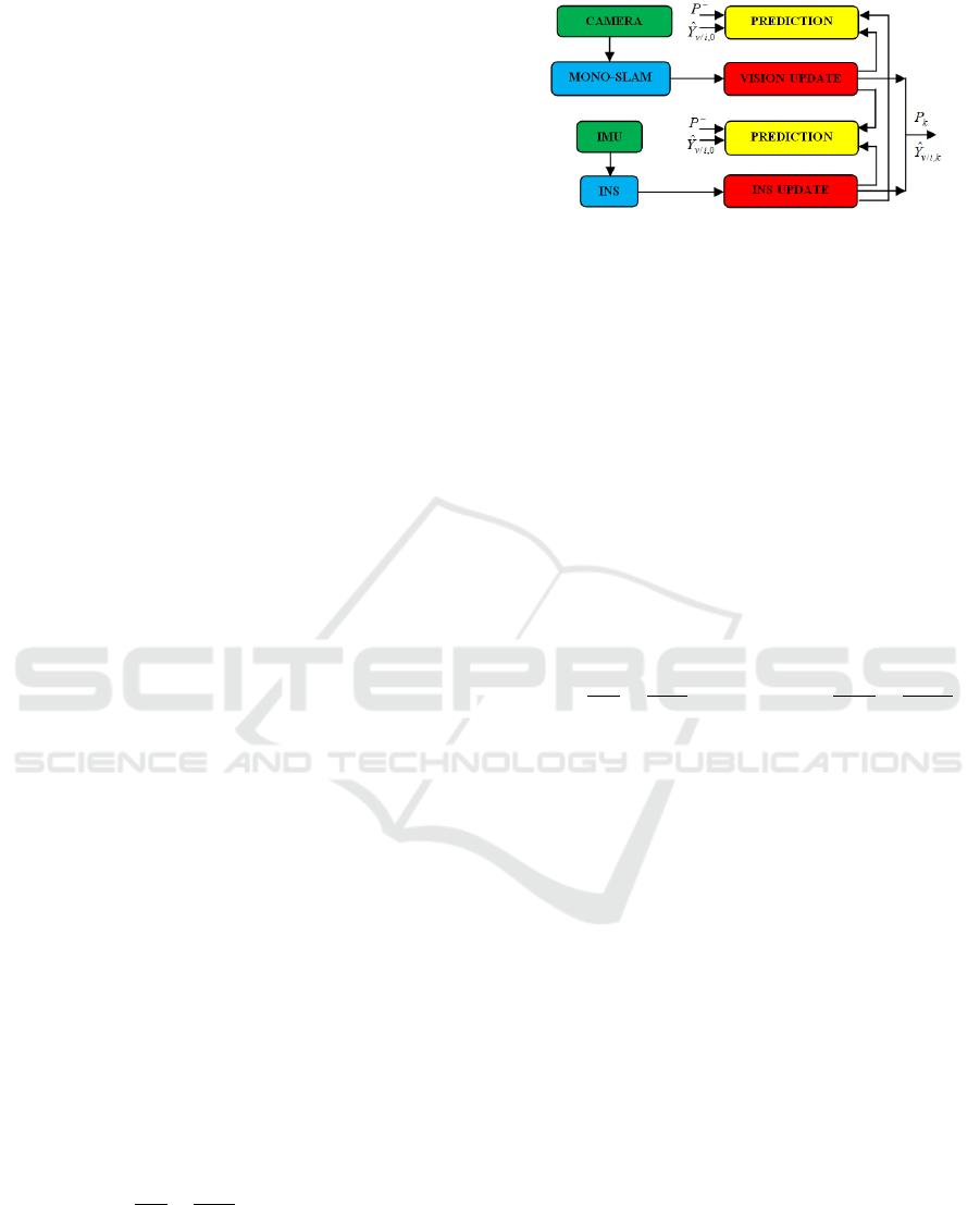
3.1.2 Synoptic Representation of the Designed
System
The system consists of two fusion processes with the
same prediction model based on a temporal motion.
The updating is realized by considering two measure-
ments coming from the Mono-SLAM and the IMU.
The transfer of state variation is alternated between
the two fusion processes into a multi rate mechnism
scheme.For more details about the designed system
see Fig. 1,
ˆ
Y
v/i,k
: represents the state vector of our
system. The notice v/i denotes vision and IMU. The
matrix P
k
is the covariance matrix, which is initialized
by P
0
.
3.2 Extended Kalman Filter Approach
The nonlinear prediction model proposed is given by:
(1). This model is detailed by the full expression
given by: (2). The scale factor is considered as an
element of the state vector which is injected in the
equations of position. For each step we get a new es-
timated scale based on the last measurement which is
used to correct the Mono-SLAM poses.
ˆ
Y
v/i,k
= f

x
k−1
,v
k−1
,a
k−1
,φ
k−1
,
˙
φ
k−1
,λ
k−1

+ q
k
(1)
ˆ
Y
k
=








I
3
T I
3
λ
k−1
T
2
I
3
2λ
k−1
0
3
0
3
0
31
0
3
I
3
T I
3
0
3
0
3
0
31
0
3
0
3
I
3
0
3
0
3
0
31
0
3
0
3
0
3
I
3
T I
3
0
31
0
3
0
3
0
3
0
3
I
3
0
31
0
13
0
13
0
13
0
13
0
13
1








ˆ
Y
k−1
(2)
Figure 1: An overview of the designed system.
The state vector elements are defined in the navi-
gation frame, where x
k
∈ R
3×1
is the position vector
without scale, v
k
∈ R
3×1
and a
k
∈ R
3×1
represent the
velocity and acceleration vectors of the Camera-IMU
system. The Euler angles are φ
k
∈ R
3×1
, the vector
˙
φ
k
∈ R
3×1
is Euler angles velocities. The parameter
λ
k
is the scale factor. The vector q
k
is a Gaussian
noise that affected our system. The index v/i defines
the prediction and the measurement in the case of vi-
sion or IMU. Where I
3
,0
3
mean an identity and zero
matrixes of dimension 3 × 3, and 0
31
,0
13
mean suc-
cessfully column and raw vectors of elements equal
to zero.
Our prediction model is a nonlinear system. Its
Jacobian matrix (F) is given by: (3).









I
3
T I
3
λ
k−1
T
2
I
3
2λ
k−1
0
3
0
3
−
T v
k−1
λ
2
k−1
−
T
2
a
k−1
2λ
2
k−1
0
3
I
3
T I
3
0
3
0
3
0
31
0
3
0
3
I
3
0
3
0
3
0
31
0
3
0
3
0
3
I
3
T I
3
0
31
0
3
0
3
0
3
0
3
I
3
0
31
0
13
0
13
0
13
0
13
0
13
1









(3)
Its prior covariance matrix is given by: (4)
P
−
= FP
k
F
T
+ Q (4)
P
−
: represents the prior covariance matrix, and
Q is the noise covariance matrix. The matrix P
k
de-
fines the posterior covariance matrix which is initial-
ized by P
0
. To involve the multi-rate mechanism, it is
suggested to consider that there are two measurement
sources (Camera and IMU). When the Mono-SLAM
box provides a new measurement, our system calcu-
lates a prediction of the state vector using the last val-
ues and doing the updating by taking into considera-
tion the Mono-SLAM data. To deal with the appro-
priate time of prediction, we use the equation (5) to
calculate the time of integration.
T = t − T
a
(5)
t: is the time of calculation defined by the loop of
execution (internal clock). The variable T
a
represents
Comparative Study between EKF, SVSF, Combined SVSF-EKF, and ASVSF Approaches based Scale Estimation of Monocular SLAM
671

the time of the last estimated vector. In case of IMU
data, the estimation process has to recover the scale
many times due to its high frequency compared to the
Mono-SLAM observation.
The two measurement models used in our paper
for the Mono-SLAM and IMU boxes are given by
equations (6) and (9) which are cited afterwards. The
state vector observation of our system is goes through
two differents observation matrices depends on mea-
surments provided by the sensor used.
Y
vm,k
= H
v
Z
SLAM,k
(6)
The observation matrix of Mono-SLAM measure-
ments is given by (7).
H
v
=

I
3
0
3
0
3
0
3
0
3
0
3×1
0
3
0
3
0
3
I
3
0
3
0
3×1

(7)
The measurement vector provided by the Mono-
SLAM box is defined by: (8).
Z
SLAM,k
=

X
SLAM,k
0
1×6
φ
SLAM,k
0
1×3
0

T
(8)
Y
im,k
= H
i
Z
IMU,k
(9)
The observation matrix of IMU measurements is
given as follows by: (10).
H
i
=

0
3
0
3
I
3
0
3
0
3
0
3×1
0
3
0
3
0
3
0
3
I
3
0
3×1

(10)
The measurement vector provided by the IMU box
is defined by: (11).
Z
IMU,k
=

0
1×6
a
IMU,k
0
1×3
˙
φ
IMU,k
0

T
(11)
The acceleration vector was calculated in the nav-
igation frame using IMU data which is given by: (12).
a
IMU,k
= C
n
b
(k − 1)a
b
IMU
+ g
n
(12)
The Euler angles velocities are defined in the nav-
igation frame by the following equation (13).
˙
φ
IMU,k
= E
n
b
(k − 1)ω
b
(k) (13)
The matrixes C
n
b
(k − 1), and E
n
b
(k − 1) represent
the cosine direction, and the rotation rate conversion
from the body to the navigation frame. g
n
is the grav-
ity in the navigation frame.
The equations of the state vector correction us-
ing Mono-SLAM data are illustrated by the following
equations: (14), (15) and (16).
K
Kalman
v,k
= P
−
k
H
T
v

H
v
P
−
k
H
T
v
+ R
v

−1
(14)
Y
v/i,k
=
ˆ
Y
v,k
+ K
Kalman
v,k

ˆ
Y
v,k
−Y
vm,k

(15)
P
k
=

I
16
− K
Kalman
v,k
H
v

P
−
(16)
The equations of state vector correction using
IMU data are illustrated by the following equations
(17), (18) and (19).
K
Kalman
i,k
= P
−
k
H
T
i

H
i
P
−
k
H
T
i
+ R
i

−1
(17)
Y
v/i,k
=
ˆ
Y
i,k
+ K
Kalman
i,k

ˆ
Y
i,k
−Y
im,k

(18)
P
k
=

I
16
− K
Kalman
i,k
H
i

P
−
(19)
Where K
Kalman
v,k
, and K
Kalman
i,k
are defined Kalman
gains for vision and IMU measurements.
The two matrixes R
v
, and R
i
are the noise covari-
ance associated with Mono-SLAM and IMU mea-
surements. The covariance matrix update is defined
by P
k
.
3.3 Smooth Variable Structure Filter
Approach
The SVSF is a closed loop filter (predictor-corrector)
proposed by S. Habibi (Habibi, 2007), developed on
the base of variable structure theory and sliding mode
concepts, its structure based principally on a prior,
and posterior errors between prediction and observa-
tion of the state vector elements.
The advantages of SVSF estimator compared to
EKF are the robustness and stability. The lineariza-
tion of the system is not needed, and the noise model
is not necessary. The disadvantages of this estima-
tor are the non optimality as all nonlinear filters, the
chattering, and the choice of the superior limit of in-
certitude.
The previous prediction model (1) and (2) is uti-
lized. The state vector elements are initialized by
Y
v/i,0
and the posterior error of estimation E
0/0
. The
update of our process is performed by using the two
considered measurements which are given by (6) and
(9). At a time, we use Mono-SLAM output, and at
another time the IMU. In this case, another observa-
tion matrixes are used H
v
= I
16
, and H
i
= I
16
, these
changes are due to the concept of SVSF mechanism.
The IMU vector measurements are given by the
following equation (20).
Z
IMU,k
=

X
IMU
V
IMU
a
IMU
φ
IMU
˙
φ
IMU
0

T
(20)
Where X
IMU,k
, V
IMU,k
, a
IMU,k
, φ
IMU,k
, and
˙
φ
IMU,k
are the position, the velocity, the acceleration, the Eu-
ler angles, and the angular rate vectors defined in the
ICINCO 2022 - 19th International Conference on Informatics in Control, Automation and Robotics
672

navigation frame. The acceleration and angular rate
vectors are synthesized using the INS mechanization
(12) and (13) based on temporal integration.
In the first process update, we use Mono-SLAM
output based on the following equations (21), (22),
(23), and (24).
E
v,k/k−1
=
ˆ
Y
v,k
−Y
vm,k/k−1
(21)
K
SV SF
v,k
= H
+
v
diag
h
(


E
v,k/k−1


Abs
+ γ


E
k−1/k−1


Abs
)
◦
sat(
¯
ψ
−1
E
v,k/k−1
)

·

diag(E
v,k/k−1
)

−1
(22)
The sign
◦
is the Schur operator (vector of element
by element multiply). Sat is the saturation function.
The notation Abs means absolute value.
Y
v/i,k/k
= Y
v,k
+ K
SV SF
v,k
E
v,k/k−1
(23)
E
k/k
=
ˆ
Y
v,k
−Y
v/i,k/k
(24)
In the second, the IMU data are utilized to update
the state vector elements based on the following equa-
tions (25), (26), (27), and (28).
E
i,k/k−1
=
ˆ
Y
i,k
−Y
im,k/k−1
(25)
K
SV SF
i,k
= H
+
i
diag
h
(


E
i,k/k−1


Abs
+ γ


E
k−1/k−1


Abs
)
◦
sat(
¯
ψ
−1
E
i,k/k−1
)

diag(E
i,k/k−1
)

−1
(26)
Y
v/i,k/k
= Y
i,k
+ K
SV SF
i,k
E
i,k/k−1
(27)
E
k/k
=
ˆ
Y
i,k
−Y
v/i,k/k
(28)
Where

E
v,k/k−1
,E
i,k/k−1

, E
k/k
define prior and
posterior errors, K
SV SF
v,k
, and K
SV SF
i,k
are the SVSF
gains calculated in case of vision and IMU obser-
vation H
+
v
, and H
+
i
are the pseudo inverses of the
two observation matrixes (Mono-SLAM and IMU)
for the vision and inertial measurements, the param-
eter γ ∈ R
16×16
(0 < γ ≤ 1) is a diagonal matrix, its
diagonal elements define the convergence rate of the
state vector elements. In our work, it is supposed the
following value γ = 0.5 × I
16
.
The diagonal matrix
¯
ψ
−1
represents the inverse of
¯
ψ. This last is a boundary constructed with respect to
the smoothing boundary layer vector.
¯
ψ
−1
=



1/ψ
1,1
· · · 0
.
.
.
.
.
.
.
.
.
0 · · · 1/ψ
16,16



(29)
3.4 Combined SVSF-EKF Approach
The SVSF is a robust estimator compared to EKF.
The author S. Habibi suggests to combine SVSF
and EKF (Habibi, 2008) to improve estimator perfor-
mance. The author, based on the variable structure
filter (VSF) enforces the estimated elements to enter
into the smooth boundary layer. Inside the boundary
layer, the EKF is involved as a primary actor of esti-
mation. We use the same model of prediction given
by (1) and (2).
The two measurement vectors provided by Mono-
SLAM and IMU boxes are similar to (6) and (9). The
observation matrices are those utilized in Sect. 3.3.
The combined SVSF-EKF gains are represented
by the following equations (30) and (31).
k
C
v,k
=

H
+
v






E
v,k/k−1


Ab
+ γ


E
k−1/k−1


Ab

+ Π



Ab

◦
sat(K
Kalman
v,k
.E
v,k/k−1
, 1)
(30)
k
C
i,k
=

H
+
i






E
i,k/k−1


Ab
+ γ


E
k−1/k−1


Ab

+ Π



Ab

◦
sat(K
Kalman
i,k
.E
i,k/k−1
, 1)
(31)
The correction of the state vector elements are cal-
culated by the following manner (32) and (33); where
K
Kalman
v,k
, and K
Kalman
i,k
are the EKF gains with respect
to vision and IMU measurements calculated by (14)
and (17). The notation Ab means absolute value.
Y
v/i,k/k
= Y
v,k
+ k
C
v,k
E
v,k/k−1
(32)
Y
v/i,k/k
= Y
i,k
+ k
C
i,k
E
i,k/k−1
(33)
It is supposed Π = 0.9 × I
16
because, this matrix
of factors defines the magnitude of EKF dominating
inside the boundary layer. It must be higher than γ in
order to emphasize Kalman action within the bound-
ary layer.
3.5 Adaptive Smooth Variable
Structure Filter Approach
An adaptive estimator version can provide better scale
estimation in terms of robustness and accuracy. The
ASVSF (Gadsden and Habibi, 2010; Gadsden et al.,
2011)( adaptive smooth variable structure filter) uti-
lizes the covariance matrix in order to have an idea
about the probability of the estimated elements. The
new version of SVSF is defined by the covariance ma-
trice derivative and an optimal boundary layer matrix
Comparative Study between EKF, SVSF, Combined SVSF-EKF, and ASVSF Approaches based Scale Estimation of Monocular SLAM
673

¯
ψ
opt
. The boundary layer matrix (29) being not diag-
onal, by including a full derivation of the covariance
matrix (Hol et al., 2007). The boundary layer
¯
ψ
opt
is
obtained by: (34), which is given by: (35).
∂(trace[P])
∂
¯
ψ
= 0 (34)
¯
ψ
opt
=



ψ
1,1
· · · ψ
1,16
.
.
.
.
.
.
.
.
.
ψ
16,1
· · · ψ
16,16



(35)
In case of ASVSF we follow the same steps de-
fined by Subsection. 3.3. The difference is in the
utilization of the covariance matrix to calculate the
boundary layer as given by (36) and (37). The correc-
tion part of the ASVSF filter needs the linearization
of the observation matrixes to calculate the optimal
boundary layer (35).
¯
ψ
opt
v,k
=

H
v
P
k
H
T
v
+ R
v

H
v
P
k
H
T
v

−1
·
h
diag



E
v,k/k−1


Abs
+ γ


E
k−1/k−1


Abs
i
(36)
¯
ψ
opt
i,k
=

H
i
P
k
H
T
i
+ R
i

H
i
P
k
H
T
i

−1
·
h
diag



E
i,k/k−1


Abs
+ γ


E
k−1/k−1


Abs
i
(37)
K
ASV SF
v,k
= H
+
v
diag
h
(


E
v,k/k−1


Abs
+ γ


E
k−1/k−1


Abs
)
◦
sat(

¯
ψ
opt
v,k

−1
E
v,k/k−1
)

·

diag(E
v,k/k−1
)

−1
(38)
K
ASV SF
i,k
= H
+
i
diag
h
(


E
i,k/k−1


Abs
+ γ


E
k−1/k−1


Abs
)
◦
sat(

¯
ψ
opt
i,k

−1
E
i,k/k−1
)

·

diag(E
i,k/k−1
)

−1
(39)
The previous gains are used in (38) and (39) to
provide the correction of state vector elements in (40)
and (41).
Y
v/i,k/k
= Y
v,k
+ K
ASV SF
v,k
E
v,k/k−1
(40)
Y
v/i,k/k
= Y
i,k
+ K
ASV SF
i,k
E
i,k/k−1
(41)
The update of the covariance matrices in the case
of vision and inertial measurement are given by: (42)
and (43).
P
k
=

I
16
− K
ASV SF
v,k
H
v

P
−

I
16
− K
ASV SF
v,k
H
v

T
+K
ASV SF
v,k
R
v
K
ASV SF
v,k
(42)
P
k
=

I
16
− K
ASV SF
i,k
H
i

P
−

I
16
− K
ASV SF
i,k
H
i

T
+K
ASV SF
i,k
R
i
K
ASV SF
i,k
(43)
4 SIMULATION RESULTS
4.1 Evaluation Scenarios
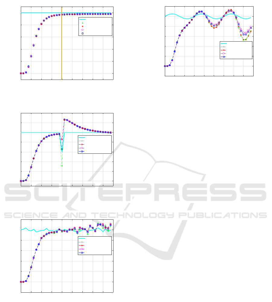
We suggest four scenarios of scale variation. At first,
an arbitrary trajectory (on Matlab software) was sim-
ulated of the couple (Camera/IMU), and it is taken
into consideration the standard deviation noises sup-
posed in Sect. 3.1. In the first scenario, the scale of
the Mono-SLAM is considered as the absolute scale
λ = 1, but we suggest a bad initialization λ
0
= 0.5
(the scale initialization is an important point of scale
estimation). The output graph is given by Fig. 2. We
remark that the absolute scale estimation (by the four
estimators) is recovered after 8 seconds despite start-
ing with a worst case. ALL approaches stabilize in the
absolute scale after 8 seconds with an average error of
0.8% due to the noises affecting the other state vec-
tor elements. In terms of approaches comparison, the
different estimators retrieve the absolute scale by al-
most the same performance despite the bad initializa-
tion. In the second scenario, it is supposed the same
steps of the previous scenario, but after scale value
stabilization λ =∼ 1 ±0.8%, an atypical value was in-
cluded (λ = 0.8) of scale to compare the robustness of
the four estimators against outliers. In Fig. 3, we no-
tice that Combined SVSF-EKF approach is more ro-
bust than EKF, SVSF, and ASVSF in front of briskly
atypical scale value. In case of scale estimation, the
ASVSF solution does not provide a good result com-
pared to Combined SVSF-EKF. This result is due to
the scale noise nature at a time, and the concept of
variable structure combined with Kalman filter in an-
other time. For a deep comparison, the ASVSF found
the scale with a performance near Combined SVSF-
EKF estimator, and also it gives the scale incertitude
for each scale value estimated. In the third scenario,
we suppose just that the Mono-SLAM output is af-
fected by a scale factor λ = 1 + n with n is a noise of
standard deviation σ
n
= 10
−4
. The aim of this sce-
nario is to show the behavior and stability of the pro-
posed approaches in front of a scale with a noise. The
result is given by Fig. 4, we see that all estimators re-
sist against scale fluctuation, and show a considerable
stability in case of scale with fulfillment to the small
standard deviation value of scale noise. To go further,
a comparison is performed later which will provide a
deep analysis about stability and robustness. It is con-
sidered in the fourth scenario, that the output of the
Mono-SLAM box is equal to the absolute scale plus
a sinusoidal variation λ = 1 + (1/40) · sin θ, with θ is
an angle of value 0 to 360 degrees. The purpose of
this scenario is to show the capability of scale track-
ing by the four estimators. The result is given by Fig.
ICINCO 2022 - 19th International Conference on Informatics in Control, Automation and Robotics
674

0 2 4 6 8 10 12 14 16 18
Time (s)
0.5
0.6
0.7
0.8
0.9
1
Scale
Absolute scale
EKF
SVSF
Combined SVSF-EKF
ASVSF
Figure 2: The first scenario of scale estimation using EKF,
SVSF, Combined SVSF-EKF, and ASVSF.
0 2 4 6 8 10 12 14 16 18
Time (s)
0.5
0.6
0.7
0.8
0.9
1
1.1
1.2
Scale
Absolute scale
EKF
SVSF
Combined SVSF-EKF
ASVSF
Figure 3: The second scenario of scale estimation using
EKF, SVSF, Combined SVSF-EKF, and ASVSF.
0 2 4 6 8 10 12 14 16 18
Time (s)
0.4
0.5
0.6
0.7
0.8
0.9
1
1.1
Scale
Absolute scale
EKF
SVSF
Combined SVSF-EKF
ASVSF
Figure 4: The third scenario of scale estimation using EKF,
SVSF, Combined SVSF-EKF, and ASVSF.
5. It is remarkable that the Combined SVSF-EKF is
more accurate than the other estimators in terms of
scale tracking. By comparison of all proposed esti-
mators, we remark that, we have not a big difference
in terms of tracking, but this difference can be signif-
icantly larger in case of the long trajectory.
0 2 4 6 8 10 12 14 16 18
Time (s)
0.4
0.5
0.6
0.7
0.8
0.9
1
1.1
Scale
Absolute scale
EKF
SVSF
Combined SVSF-EKF
ASVSF
Figure 5: The fourth scenario of scale estimation using
EKF, SVSF, Combined SVSF-EKF, and ASVSF.
4.2 Performances Analysis
We try to give an indepth analysis of the proposed es-
timators for scale estimation in terms of robustness,
stability, and accuracy based on the appropriate mea-
surement tools.
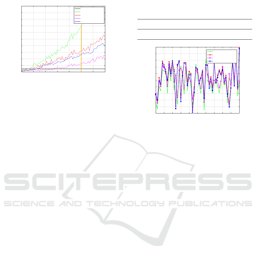
4.2.1 Robustness and Stability Analysis
To assess the robustness and stability measurement
(Maronna et al., 2006) of each estimator, the fol-
lowing manner is adopted; the Mono-SLAM scale is
supposed to be affected by noise of standard devia-
tion σ
n
= 10
−4
. A point is selected in the middle of
scale estimation process (this point has a typical scale
around the absolute scale), this last was changed by an
atypical scale. The value of this outlier is augmented
gradually until 100 percent of the scale contamina-
tion. The experience is repeated many times to get
significant results. At the end, we measure the maxi-
mum bias of scale deviation compared to the absolute
scale for the four estimators using the formula (44).
λ
Max
b
= max


λ
i
− λ
Re f


(44)
Where λ
Re f
is the scale reference without contam-
ination, and λ
Max
b
signifies the bias max of scale devi-
ation of a given contamination, the term λ
i
is the scale
value in the case of the same contamination measured
many times (i times). The results are given by the
graph in Fig. 6. It is remarkable that, all the estima-
tors involved in scale recovering lost their robustness
significantly according to scale contamination until
instability of scale recovery process. The best estima-
tor in terms of robustness is the Combined SVSF-EKF
due to the synergy provided by the couple SVSF-
EKF. After, comes the ASVSF because it has the vari-
able structure force with an optimal gain ensured by
the variable boundary layer. The SVSF presents also
a significant robustness under the ASVSF but better
than the classical solution (EKF). The maximum scale
Comparative Study between EKF, SVSF, Combined SVSF-EKF, and ASVSF Approaches based Scale Estimation of Monocular SLAM
675

0 10 20 30 40 50 60 70
Scale contamination (Percents)
0
0.2
0.4
0.6
0.8
1
1.2
1.4
1.6
1.8
2
Bias Max of scale
Break Point level
EKF
SVSF
Combined SVSF-EKF
ASVSF
Figure 6: The robustness and stability analysis of EKF,
SVSF, Combined SVSF-EKF, and ASVSF.
bias deviation allowed by scale recovery process de-
pends on the application. However, in our work, we
suggest that the bias max of scale tolerance is equal
to 0.1. It is remarkable that the Combined SVSF-
EKF has the best break point which is around 30%,
the ASVSF is about 15%, the SVSF is approximately
10%, and EKF is under 10%. Beyond these scale con-
taminations’ values, the robustness of the proposed
estimators are not guaranteed with respect to the max-
imum scale deviation supposed. In case of scale con-
tamination of 50 percent, the maximum deviation of
scale bias deviation does not exceed 0.3 for the Com-
bined SVSF-EKF approach. In case of ASVSF, the
deviation is approximately 0.5, for SVSF is about
0.6, and in the classical method the maximal devia-
tion of scale bias is 1.4 (this means instability of the
scale method). For the robust filter (SVSF, Combined
SVSF-EKF, and ASVSF) the stability of our system is
guaranteed compared to the EKF approach. But, it is
recommended to select the ASVSF estimator, because
it brings together many advantages as the robustness,
the accuracy, the uncertainty information, and the re-
spect of the real time constraint.
4.2.2 Accuracy Analysis
To analyze the accuracy and to give a quantification of
the precision range of our methods, we try to measure
the accuracy of the suggested estimators by consider-
ing the following steps. The scale is affected by noise
of a standard deviation σ
n
= 10
−4
. Some points of
the scale estimation system are replaced by outliers
near scale tolerance (these scale values can be sup-
ported easily by our proposed system) of value equal
to 0.12 (in these points the scale becomes λ = 0.88).
The number of points touched by scale outliers is in-
creased gradually to 100 percent. For each contami-
nation, we calculate the corresponding average of the
root-mean-square error (RMSE). The graph of accu-
racy measurement is given by Fig. 7. It is remarkable
Table 1: The means RMSE of EKF, SVSF, Combined
SVSF-EKF, and ASVSF.
Est EKF SVSF Combined ASVSF
Mean 0.084 0.086 0.085 0.086
0 10 20 30 40 50 60 70 80 90 100
Percentage of Outliers (Percents)
0.074
0.076
0.078
0.08
0.082
0.084
0.086
0.088
0.09
0.092
0.094
RMSE
EKF
SVSF
Combined SVSF-EKF
ASVSF
Figure 7: The accuracy analysis of EKF, SVSF, Combined
SVSF-EKF, and ASVSF.
that the Combined SVSF-EKF is near optimal perfor-
mance of the famous estimator EKF. There is not a
big difference between SVSF and ASVSF in terms of
accuracy, so it depends on the application in which it
is involved (in case of searching for high precision).
The graph of RMSE in case of ASVSF is near to the
Combined SVSF-EKF, so it is preferable to select the
ASVSF instead of the Combined SVSF-EKF despite
the superiority presented because, at least the ASVSF
provides an idea about the uncertainty of the scale
value. To understand better the Fig. 7, the Table 1 is
proposed which gives a summary of the means RMSE
for the four estimators proposed. The RMSE of all
the estimators is numerically close, but in case of the
scale value, the least difference is considerable.
5 EXPERIMENT RESULTS
5.1 The Environment of Experiment
The experiment results are realized by using a
dataset of a micro aerial vehicle (MAV) (an As-
cTec Firefly hex-rotor helicopter). This MAV has
two monochrome front-down looking Cameras type
MT9V034 of a rate 20 Hz and an IMU type
ADIS16448 of MEMS technology with a rate of 200
Hz. The standard deviations of noises, biases, and the
frequencies of IMU are given in the Methodology sec-
tion. For more details about the system configuration,
refer to (Burri et al., 2016).
ICINCO 2022 - 19th International Conference on Informatics in Control, Automation and Robotics
676

-3 -2 -1 0 1 2 3 4 5 6
X (m)
-4
-2
0
2
4
6
8
10
Y (m)
Ground truth
Mono-SLAM trajectory
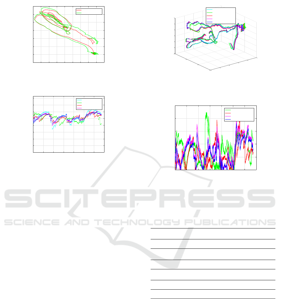
Figure 8: The top view of the trajectory obtained by the
Mono-SLAM and the ground truth in case of a real data
(MH 01 easy).
0 50 100 150 200 250 300 350
Time (s)
0.5
0.6
0.7
0.8
0.9
1
1.1
1.2
1.3
Scale
Scale of Mono-SLAM
EKF
SVSF
Combined SVSF-EKF
Figure 9: The scale estimation using EKF, SVSF, Combined
SVSF-EKF and ASVSF in case of a real data (MH 01 easy).
5.2 The Scale Recovering of a Real Data
To obtain the up to scale trajectory, we applied on
the image of the dataset a well known Mono-SLAM
named inverse depth parameterization for monocular
SLAM (Civera et al., 2008). This Mono-SLAM is
based essentially on the EKF. The brute force of this
solution is the representation of the depth by its in-
verse form. However, it allows to handle uncertainty
accurately during undelaying initialization and be-
yond. As all kinds of Mono-SLAM, it provides a tra-
jectory with an unknown scale as given by Fig. 8. We
applied the fourth proposed estimators to recover the
absolute scale on this up to scale trajectory as given by
Fig. 9. This figure shows the superiority of scale re-
covering of the robust filter against the classical solu-
tion (EKF). The Fig. 10 shows the 3D trajectory of the
MAV (ground truth) and the estimated trajectories re-
alized by the four estimators (EKF, SVSF, Combined
SVSF-EKF and ASVSF) in case of a real data (MH
01 easy). To provide a clear comparison between all
the estimators, we suggest to calculate the RMSE for
all these estimators as given by Fig. 11. The robust
filter provides a good result in term of scale tracking
in case of real data. This judgment stays valid for the
other scenarios choices from the dataset (MH 01 easy,
MH 03 medium, and MH 05 difficult) as given by the
Table 2. The RMSE for the four estimators degraded
systematically by the quality of frames acquired from
the explored environment, this limitation is due to the
-1.5
10
-1
-0.5
6
0
Z (m)
5
0.5
4
Y (m)
1
2
X (m)
1.5
0
0
-2
-5
-4
Ground truth
EKF
SVSF
Combined SVSF-EKF
ASVSF
Figure 10: The 3D trajectories of ground truth, EKF, SVSF,
Combined SVSF-EKF and ASVSF in case of a real data
(MH 01 easy).
0 1000 2000 3000 4000 5000 6000 7000
Iteration
0
0.05
0.1
0.15
0.2
0.25
Error (m)
EKF
SVSF
Combined SVSF-EKF
ASVSF
Figure 11: The RMSE of trajectories for EKF, SVSF, Com-
bined SVSF-EKF and ASVSF in case of a real data (MH 01
easy).
Table 2: The mean RMSE of scale estimation using EKF,
SVSF, Combined SVSF-EKF, and ASVSF in case of a real
data (MH 01 easy, MH 03 medium, and MH 05 difficult)
MH 01 MH 03 MH 05
Length (m) 80.6 130.9 97.6
Duration (s) 182 132 111
Mean EKF 0.0857 0.0987 0.0997
Mean SVSF 0.0590 0.0773 0.0882
Mean Combined 0.0319 0.0468 0.0643
Mean ASVSF 0.0425 0.0564 0.0725
high perturbation of scale which is affected by the low
textured or darkness of frames acquired.
5.3 The Real Time Evaluation
The environment of development is Matlab, installed
into a computer of a characteristic; Intel(R) Core
(TM), processor i5 of frequency 2.40 GHz. In our
work, the scale is recovered into a multi-rate mecha-
nism. However, the Mono-SLAM utilized in our work
provides an up to scale trajectory in real time of fre-
quency 20 Hz. Our solutions permit to estimate the
Comparative Study between EKF, SVSF, Combined SVSF-EKF, and ASVSF Approaches based Scale Estimation of Monocular SLAM
677

Table 3: The frequency of scale estimation for EKF, SVSF,
Combined SVSF-EKF, and ASVSF
Est EKF SVSF Combined ASVSF
Freq 93 Hz 105 Hz 88 Hz 97 Hz
scale many times between two poses, this mean that
it is possible to do another estimation stage in a pe-
riod of about 50 ms. From the Table 3, we note that
the scale value is improved within a frequency big-
ger than the vision part. But, this frequency, depends
essentially on the mathematical formulation for each
estimator. The frequency of estimation can not be
evaluated separately from the scale estimation quality.
Sure, that SVSF is the better in terms of frequency,
but, it is not the best in term of RMSE. The Com-
bined SVSF-EKF is a good estimator but also it is
not the fastest. The ASVSF can be considered as a
good estimator of scale because it allows to recover
the scale in real time with a rate of about 97 Hz and a
scale near Combined SVSF-EKF quality.
6 CONCLUSIONS
This paper focused on a timely problem which relies
to the Mono-SLAM field. It treats the scale recov-
ering into a multi-rate fusion scheme. We have im-
plemented, and compared four approaches of scale
estimation: EKF, SVSF, Combined SVSF-EKF, and
ASVSF. The obtained results of this work, showed a
significant performance of robust filters (SVSF, Com-
bined SVSF-EKF, and ASVSF) against the classical
solution (EKF) in terms of scale factor recovering
and real time constraint. The different results ob-
tained permit to focus on the Combined SVSF-EKF
method which provides a compromise between ro-
bustness and accuracy. But, in terms of real time
constraint, it is better to utilize the ASVSF estima-
tor. In addition, the ASVSF is near performance of
the Combined SVSF-EKF, and also it provides an as-
sesses about the incertitude of scale estimation as in
the case of the EKF. In this work, we showed that the
filtering process into multi-rate mechanism allows the
determination of the scale factor with a rate superior
than the vision system 20 Hz especially for SVSF, and
ASVSF. As a future work, we plan to design from
scratch a new Mono-SLAM system with some new
ideas and to involve our solution to estimate the scale.
The complete system can be embedded easily onto a
MAV in order to navigate safely. In the same subject
studied in this paper, we propose to design another
system by many sensors and studying the fault toler-
ance of the developed system.
REFERENCES
Agrawal, M. and Konolige, K. (2006). Real-time localiza-
tion in outdoor environments using stereo vision and
inexpensive GPS. In International Conference on Pat-
tern Recognitionon, pages 1063–1068.
Armesto, L., Chroust, S., Vincze, M., and Tornero, J.
(2004). Multi-rate fusion with vision and iner-
tial sensors. In Robotics and Automation, Proceed-
ings. ICRA’04 International Conference on, volume 1,
pages 193–199. IEEE.
Botterill, T., Mills, S., and Green, R. (2013). Cor-
recting scale drift by object recognition in single-
camera SLAM. IEEE transactions on cybernetics,
43(6):1767–1780.
Burri, M., Nikolic, J., Gohl, P., and Schneider, T. (2016).
The euroc micro aerial vehicle datasets. The Inter-
national Journal of Robotics Research, 35(10):1157–
1163.
Civera, J., Davison, A., and Montiel, J. (2008). Inverse
depth parametrization for monocular SLAM. IEEE
transactions on robotics, 24(5):932–945.
Davison, A., Reid, I., and Molton, N. (2007). Mono SLAM:
Real-time single camera SLAM. IEEE Transactions on
Pattern Analysis & Machine Intelligence, (6):1052–
1067.
Dumortier, Y., Benenson, R., and Kais, M. (2006). Real-
time vehicle motion estimation using texture learning
and monocular vision. In International Conference on
Computer Vision and Graphics ICCVG.
Eade, E. and Drummond, T. (2006). Scalable monocu-
lar SLAM. In Computer Vision and Pattern Recog-
nition, 2006 IEEE Computer Society Conference on,
volume 1, pages 469–476. IEEE.
Engel, J. and Cremers, D. (2014). Lsd-SLAM: Large-scale
direct monocular SLAM. In European Conference on
Computer Vision, pages 834–849. Springer.
Forste, C., Lynen, S., Kneip, L., and Scaramuzza, D.
(2013). Collaborative monocular SLAM with multiple
micro aerial vehicles. In International Conference on
Intelligent Robots and Systems on, pages 3962–3970.
IEEE.
Frost, D., Kahler, O., and Murray, D. (2016). Object-
aware bundle adjustment for correcting monocular
scale drift. In Robotics and Automation (ICRA), In-
ternational Conference on, pages 4770–4776. IEEE.
Gadsden, S. and Habibi, S. (2010). A new form of
the smooth variable structure filter with a covariance
derivation. In Decision and Control (CDC), 49th Con-
ference on, pages 7389–7394. IEEE.
Gadsden, S., Sayed, M. E., and Habibi, S. (2011). Deriva-
tion of an optimal boundary layer width for the smooth
variable structure filter. In American Control Confer-
ence (ACC), pages 4922–4927. IEEE.
Grater, J., Schwarze, T., and Lauer, M. (2015). Robust scale
estimation for monocular visual odometry using struc-
ture from motion and vanishing points. In Intelligent
Vehicles Symposium (IV), 2015 IEEE, pages 475–480.
IEEE.
ICINCO 2022 - 19th International Conference on Informatics in Control, Automation and Robotics
678

Gutierrez-Gomez, D., Puig, L., and Guerrero, J. (2012).
Full scaled 3d visual odometry from a single wear-
able omnidirectional camera. In Intelligent Robots
and Systems (IROS), RSJ International Conference
on, pages 4276–4281. IEEE.
Habibi, S. (2007). The smooth variable structure filter. Pro-
ceedings of the IEEE, 95(5):1026–1059.
Habibi, S. (2008). Combined variable structure and Kalman
filtering approach. In American Control Conference,
2008, pages 1855–1862. IEEE.
Hol, J., Schon, T., Luinge, H., and Gustafsson, F. (2007).
Robust real-time tracking by fusing measurements
from inertial and vision sensors. Journal of Real Time
Image Processing, 02(02):149–160.
Ikeda, S., Sato, T., and Yamaguchi, K. (2007). Construction
of feature landmark database using omnidirectional
videos and GPS positions. In International Confer-
ence on Pattern Recognitionon, pages 249–256. IEEE.
Jung, S. and Taylor, C. (2001). Camera trajectory estimation
using inertial sensor measurements and structure from
motion results. In Proceedings of the IEEE Computer
Society Conference on Computer Vision and Pattern
Recognition, pages 732–737.
Kitt, B., Rehder, J., Chambers, A., and Schonbein, M.
(2007). Monocular visual odometry using a planar
road model to solve scale ambiguity. In Proc of Euro-
pean Conference on Mobile Robots.
Klein, G. and Murray, D. (2007). Parallel tracking and
mapping for small ar workspaces. In Mixed and Aug-
mented Reality, ISMAR, 6th IEEE and ACM Interna-
tional Symposium on, pages 225–234. IEEE.
Kobzili, E., Larbes, C., and Allam, A. (2017a). Multi-rate
robust scale estimation of monocular SLAM. In Sys-
tems and Control (ICSC), 6th International Confer-
ence on, pages 1–5. IEEE.
Kobzili, E., Larbes, C., and Allam, A. (2017b). Robust
absolute scale estimation of monocular SLAM using
a combined svsf-ekf strategy for mav navigation. In
1st Algerian Multi-Conference on Computer, Electri-
cal and Electronic Engineering. USTHB of Algiers.
Lemaire, T., Berger, C., Jung, I., and Lacroix, S.
(2007). Vision-based SLAM: Stereo and monocular
approaches. International Journal of Computer Vi-
sion, 74(3):343–364.
Lothe, P. (2010). Simultaneous localization and mapping
with monocular vision constraint with SIG. PhD the-
sis, University of Blase Pascal Clermont-Ferrand II,
France.
Maronna, R., Martin, R., and Yohai, V. (2006). Robust
statistics. Wiley Chichester.
Montemerlo, M. (2003). A factored solution to the simul-
taneous localization and mapping problem with un-
known data association. Ph. D. thesis, Carnegie Mel-
lon University, Pittsburgh.
Mur-Artal, R., Montiel, J., and Tardos, J. (2015). Orb-
SLAM: a versatile and accurate monocular SLAM sys-
tem. IEEE Transactions on Robotics, 31(5):1147–
1163.
Nemra, A. (2011). Robust airborne 3d visual simultane-
ous localisation and mapping. Ph. D. thesis, Cranfield
University, England.
Nister, D., Naroditsky, O., and Bergen, J. (2006). Visual
odometry for ground vehicle applications. Journal of
Field Robotics, 23(1):3–20.
Nutzi, G., Weiss, S., Scaramuzza, D., and Siegwart, R.
(2011). Fusion of imu and vision for absolute scale
estimation in monocular SLAM. Journal of intelligent
& robotic systems, 61(1-4):287–299.
Pillai, S. and Leonard, J. (2015). Monocular SLAM sup-
ported object recognition. In Computer Vision and
Pattern Recognition.
Pirker, K., R
¨
uther, M., and Bischof, H. (2011). Cd SLAM-
continuous localization and mapping in a dynamic
world. In Intelligent Robots and Systems (IROS), 2011
IEEE/RSJ International Conference on, pages 3990–
3997. IEEE.
Qiang, L., Jianye, M., Guosheng, W., and Huican, L.
(2016). Absolute scale estimation of orb-SLAM al-
gorithm based on laser ranging. In Robotics and Au-
tomation (ICRA), International Conference on, pages
10279–10283. IEEE.
Scaramuzza, D., Fraundorfer, F., Pollefeys, M., and Sieg-
wart, R. (2009). Absolute scale in structure from mo-
tion from a single vehicle mounted camera by exploit-
ing nonholonomic constraints. In Computer Vision,
12th International Conference on, pages 1413–1419.
IEEE.
Scaramuzza, D. and Siegwart, R. (2008). Appearance-
guided monocular omnidirectional visual odometry
for outdoor ground vehicles. IEEE transactions on
robotics, 24(5):1015–1026.
Simond, N. and Rives, P. (2004). Trajectography of an
uncalibrated stereo rig in urban environments. Intel-
ligent Robots and Systems, 2004.(IROS 2004). Pro-
ceedings. 2004 IEEE/RSJ International Conference
on, (4):3381–3386.
Smith, R., Self, M., and Cheeseman, P. (1990). Estimat-
ing uncertain spatial relationships in robotics. In Au-
tonomous robot vehicles, pages 167–193. Springer.
Song, S. and Chandraker, M. (2014). Robust scale estima-
tion in real-time monocular sfm for autonomous driv-
ing. In Proceedings of the IEEE Conference on Com-
puter Vision and Pattern Recognition, pages 1566–
1573.
Strelow, D. and Singh, S. (2004). Motion estimation from
image and inertial measurements. International Jour-
nal of Robotique Research, 23(12):1157–1195.
Weiss, S. and Siegwart, R. (2011). Real-time metric state
estimation for modular vision-inertial systems. In
International Conference on Robotics and Automa-
tion:(ICRA 2011), pages 4531–4537. IEEE.
Zachariah, D. and Jansson, M. (2011). Self-motion and
wind velocity estimation for small-scale uavs. In
Robotics and Automation (ICRA), International Con-
ference on, pages 1166–1171. IEEE.
Comparative Study between EKF, SVSF, Combined SVSF-EKF, and ASVSF Approaches based Scale Estimation of Monocular SLAM
679