Power System Operation Modeling, Monitoring and Control
using Petri Nets
Milton Bastos de Souza
1 a
, Evangivaldo Almeida Lima
2 b
and J
`
es Jesus Fiais Cerqueira
3 c
1
´
Area Automac¸
˜
ao Industrial, Campos Integrado de Manufatura e Tecnologias Senai-Cimatec, Bahia, Salvador, Brazil
2
Exact Sciences Department, State University of Bahia, Salvador, Brazil
3
Electrical Engineering Department, Polytechnic of Federal University of Bahia, Salvador, Brazil
Keywords:
Petri Nets, Electric Power System, Modelling, Monitoring, Control, Circuit Breaker, Disconnect Switch.
Abstract:
Petri nets have been widely used as a tool for the model of Dynamics Discrete Event System (DDES). In this
paper, Petri nets are used to model, monitor and control Electrical Power Operation (EPO). For that, it will be
used a linear transformation to expand the original Petri net. The expansion will change the original rules of
firing transitions. Its changes impose restrictions on the system’s operation. As result, a simplified equation is
presented and it is used for monitoring and controlling EPO.
1 INTRODUCTION
In the earlier years, Power Systems Operations (PSO)
have been analyzed using logic diagrams to sta-
ble functionalities rules for their ways of operation.
Nowadays, have been used modern tools for analy-
sis and control that have not been used for this action
before. One of these tools is Petri nets (PN) (Tekiner-
Mogulkoc et al., 2012).
Generally, in the study of a PSO is considered that
its operation should occur predominantly in a steady
state. In this case, all the load changes, provoked
by the operation or not of the circuit breaker or any
other occurrence that can generate transients in the
power system are not considered. Thus, all variables
are manipulated with dependence only on time in the
strictly mathematical sense (Weiss and Schulz, 2015).
However, when the dynamic of operation of a PSO is
analyzed its operation can be considered as a system
whose dynamic is event-driven, i.e. it can be manipu-
lated as a Discrete Event System (DES) (Amini et al.,
2019).
Originally, a system is considered as a Dynamic
Discrete Event System (DDES) if its dynamic is such
that it can be considered as having no dependence on
time, but it is considered as having dependence on oc-
currences or events. The elapsed time of the event is
a
https://orcid.org/8265-2459-2141-3657
b
https://orcid.org/3664-7680-0086-3560
c
https://orcid.org/0000-0003-4072-0101
usually negligible. There are several tools used in the
study DES for different kinds of systems. Among the
main tools used in the study of DES, one can point
out Finite State Automata, Dioids, Queue Theory, and
Petri Nets (Papadopoulos et al., 2019; Wu et al., 2019;
Komenda et al., 2018; Lin et al., 2016).
The Petri nets are as well known in the DES analy-
sis and its popularity comes mainly due to two factors:
its compact representation and its graphic representa-
tion. Over time, the Petri nets have been incorporat-
ing several resources to become them, more powerful
(Murata, 1989; David and Alla, 1994; Bin et al., 2015;
Fendri and Chaabene, 2019).
In this work, Petri nets are used for monitoring
and synthesis of controllers for PSO. Using matrix al-
gebra and supervisory control theory a Petri nets is
used to model Power System Operation (Giua, 1992;
Krogh and Holloway, 1991; Holloway et al., 1996;
Dideban and Alla, 2009).
This work is complemented with the following
sections: Theoretical background composed by Petri
nets concepts and a little review of Power System Op-
eration. In the following section, the use of Petri nets
in the Power System Operation is presented as the
tool for modeling. After that, the original model is
expanded to monitoring and control. The section Ap-
plication is used to validate the theory presented in
the preview sections. The Conclusion Section are pre-
sented the mains results (Souza et al., 2016).
658
Bastos de Souza, M., Lima, E. and Cerqueira, J.
Power System Operation Modeling, Monitoring and Control using Petri Nets.
DOI: 10.5220/0011314400003271
In Proceedings of the 19th International Conference on Informatics in Control, Automation and Robotics (ICINCO 2022), pages 658-667
ISBN: 978-989-758-585-2; ISSN: 2184-2809
Copyright
c
 2022 by SCITEPRESS – Science and Technology Publications, Lda. All rights reserved

2 THEORETICAL BASIS
2.1 Petri Nets
A Petri net is a particular kind of directed bipartite
graph (or digraph) together with an initial state called
the initial marking. It contains two types of nodes,
places and transitions. In the graphical representa-
tion, places are drawn as circles, and transitions as
bars or boxes. Arcs links either from a place to a tran-
sition or from a transition to a place. Arcs are labeled
with their weights (positive integers). Labels for unity
weight are usually omitted. A marking (state) assigns
to each place(p) is a non-negative integer k; we say
that p is marked with k tokens. Pictorially, we place k
black dots (tokens) in place p. If k is large, it can sim-
ply write the number k inside p to represent k tokens.
A marking is denoted by M, an m-vector, where m is
the total number of places. The number of marks in-
side p are denoted by ]M. (Murata, 1989; David and
Alla, 1994; Cassandras and Lafortune, 2009).
Definition 1. A PN is a five-tuple PN =
(P,T,I,O,M
0
), where
1. P = {p
1
, p
2
,. .. , p
m
} is a finite set of places.
2. T = {t
1
,t
2
,. .. ,t
n
} is a finite set of transitions, P∪
T 6=
/
0,P ∩T =
/
0
3. B
−
: PT → N is an input matrix such that its el-
ements defines the directed arcs from places to
transitions, where N = {0, 1, 2,. ..}.
4. B
+
: PT → N is an output function that defines the
directed arcs from transitions to places.
5. M : P → N is a marking vector representing the
numbers of tokens in places with Mo denoting the
initial marking.
In modeling, often places represent conditions and
transitions represent events. A transition (event) has
a certain number of input and output places repre-
senting the preconditions and postconditions, respec-
tively. The presence of a token in places are inter-
preted as the truth of the condition associated with
places.
2.1.1 Enabling and Firing Rules
Definition 2. A PN is said to be an ordinary PN if
for any arc in the net its weight is 1. The preset of
transition t is the set of all input places to t, i.e., •t =
{p : p ∈ P and B
−
(p,t) > 0}. The postset of t is the
set of all output places from t, i.e., t
•
= {p : p ∈ P
and B
+
(p,t) > 0}. Similarly, the preset of p is •p =
{t : t ∈ T : B
+
(p,t) > 0} and postset p• = {t : t ∈ T :
B
−
(p,t) > 0}.
Definition 3. A transition t ∈ T in PN is enabled in
marking M if for all p ∈ •t,
M(p) ≥ B
−
(p,t)
If a transition is enabled, it can fire. Firing an enabled
transition t in marking M yields
M
0
(p) =



M(p) −B
−
(p,t), if p ∈ t
M(p) +B
+
(p,t), if p ∈ t
M(p), if otherwise
2.2 Power Systems Elements: Models
Electric Power Systems(EPS) are a set of equipment
that operates in a coordinated manner with the pur-
pose of providing electricity to consumers, within
certain standards of quality (reliability, availability),
safety and costs, with minimal environmental im-
pact.They share and contribute to the progress and
technological advances of humanity. The growth in
electricity consumption in the world is considered
phenomenal. This makes the EPS increasingly larger
and consequently increases the complexity. Typically,
electrical power systems can be divided into three
large blocks:
Generation - Performs the function of converting
some form of energy (hydraulic, thermal, etc.)
into electrical energy;
Transmission - Responsible for transporting elec-
tric energy from Production Centers to Consumer
Centers, or even other electrical systems, inter-
connecting them;
Distribution - Distributes the electricity received
from the transmission system to large, medium
and small consumers.
Therefore, the electrical system, as a whole, consists
of multiple generation sources that are used to serve
the load centers, a process that is done by complex
transmission systems. From the above, to keep this
complex system operating properly, with quality and
safety standards, it is necessary, therefore, monitoring
and control.
As modelling tool, Petri Nets can be used to model
Power System Operation. To do that, it is neces-
sary limit the constructive characteristics of its com-
ponents. therefore, the degree of complexity of the
circuit breaker should consider the following internal
components:
1. Axillary contacts
2. Main contacts
3. Protective cover for arc contacts
4. Porcelain wrap
Power System Operation Modeling, Monitoring and Control using Petri Nets
659

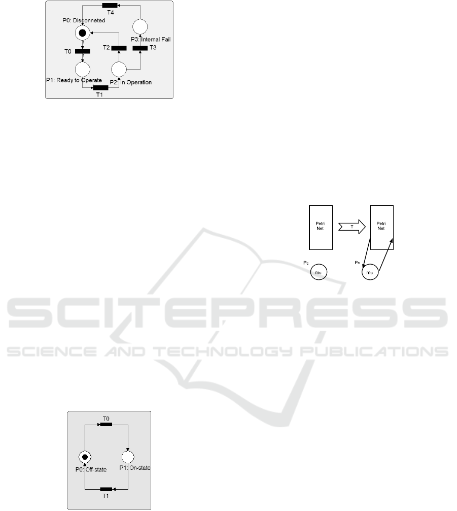
Figure 1: Circuit Breaker Model Using PN.
The states to put in its model will be
In Operation - when the circuit breaker is in the on
state
Disconnected - when the circuit breaker is in the off
state
Ready to Operate - when the circuit breaker spring
is charging
Internal Fail - When the breaker trips because of an
internal failure
The circuit breaker operation occur after it is ready
to operate. Regarding the shutdown, it can be turned
off manually or automatically due to internal failure
being recovered ready to restart . So the way to rep-
resent the circuit breaker via Ordinary Petri is shown
below in the Figure 1.
The electric power generator and disconnect
switch in this paper will be modeled in two states. In
the on-state, the generator and disconnect switch is
supplying energy and transferring power respectively.
The off-state, the generator shuts down and the dis-
connect switch suspends transference. In the Figure 2
is shown the Petri Net of these components.
Figure 2: Petri Net Model for Generator and Disconnect
Switch.
2.3 Expansion of Petri Net
In this chapter the use of PN will be introduced in
the study of the operation of an EPS. Initially, an PN
will be expanded with the addition, in its structure, of
one or more places and its consequent transformation
from an autonomous to a non-autonomous PN. At the
end of this transformation, issues related to monitor-
ing, control and diagnosis will be studied.
A Place-Transition type Petri net, autonomous,
containing m places and n transitions and with ini-
tial marking M
0
. The Petri net can be added with
some places (pci) with M
ci
marking, however, follow-
ing some premises, which are dictated by the interest
in the expansion. In this paper, given the expansion of
PN, it is interesting to guarantee two basic premises:
• The marking of the original network must be guar-
anteed
• The number of marks of the incorporated place
should be related to the mark of the original net-
work
The Figure 3 shows a block diagram of the expanded
Petri Net. From a graphical point of view, this expan-
Figure 3: Petri Net Expansion Block Diagram.
sion can be interpreted as shown in Figure 3. The
Petri net gains a new place, therefore, the connec-
tion between the new place and the old PN must be
through arcs from the new place to PN transitions and
from the transitions of the PN to the new place. From
the algebraic point of view, the transformation corre-
sponds to an expansion of matrices, that is, a linear
transformation over matrices, as seen below
T :

M ⇒ M
h
N
(m)
⇒ N
(m+1)
The transformed matrix M
h
will then be of the
form:
M
h
= AM
The order of A being as, [A]
(m+1)×m
. Matrix A can be
broken down into two parts, each part meeting one of
the premisses:
A =


A
1
.. .
A
2


(1)
So that, it can find the the result in the Equation(2):
M
h
=


A
1
.. .
A
2


M =


A
1
M
.. .
A
2
M


(2)
where,
ICINCO 2022 - 19th International Conference on Informatics in Control, Automation and Robotics
660

• A
1
.M corresponding to marking the old PN. Thus
A
1
is the identity matrix of order equal to the num-
ber of lines of M, that is, A
1
= [I]
m×m
.
• A
2
.M is the number of outside place marks and the
vector A
2
will be treat as the vector line C, whose
order will be [C]
1×m
.
• C = [c
1
,c
2
,. .. ,c
m−1
,c
m
]
T (M) = M
h
=


I
m
.. .
C


M =


I
m
M
.. .
CM


(3)
Denoting ]M, number of marks in the in the old PN;
]T (M) = ]M + ]M
c
(4)
The element M in the Equation(2), can involve only
a portion of the places marked in the PN, hence Im
is replaced by its main diagonal L, containing L(i, i)
belongs to N as desired whether or not the place in
the desired operation. Thus, L(i) = Im(i, i) = 1, 2,. ..
means that the place p (i) is included in the desired
operation, otherwise L (i) = 0. Taking the vector line
L, the Equation(4), of the number of marks of the ex-
tended PN becomes, see Equation(5)
]T (M) = ]LM + ]CM = ]


L
.. .
C


M (5)
the Equation(5) allows computing the number of
marks to the external place from a value of the orig-
inal PN. Once the transformation is known, the dy-
namics of the expanded PN is evaluated, that is, how
the state of the new PN changes. The Marking of ex-
panded PN will be,
]M
h
= ]T (M) = LM +CM (6)
However, considering the dynamics. of the original
Petri net, this means that the PN remains autonomous,
that is, the presence of the external place does not in-
terfere with the change of state of the original PN.
From the Original equation,
M = M
0
+ Bq
And using the expansion matrices, A, is find that:
M
h
= AM
o
+ABq =


L
.. .
C


M
0
+


L
.. .
C


Bq (7)
being,
M
h
= M
ho
+ABq =


L
.. .
C


M
0
+


L
.. .
C


Bq (8)
Until then, the PN remains autonomous. obeying only
the rules of formalism, the place p
c
just observes,
monitors, watches. The next step, then, is to deter-
mine the markup value of the inserted place and its
incidence matrix, that is, (M
co
, CB). The equations
above allow, therefore, to analyze an expanded PN of
a place without losing the information of the PN. This
analysis will be extended to the following themes:
• System Monitoring
• Supervisory Control
• Partial Observation by the Controller
• Fault Diagnosis
2.3.1 PSO Monitoring using Petri Net
However advanced, from a technological point of
view, systems are subject to disturbances in their dy-
namics. These disturbances can be caused by external
or internal sources and can cause problems of differ-
ent orders. Thus, it is essential to monitor or supervise
the systems. Condition for monitoring the system us-
ing PN as a model. In this paper, it will use external
places to monitor one or more places in a Petri net.
The following boundary condition will be accepted,
see Equation(9)
CM − LM = 0 (9)
The above equation is equivalent to Equation(10).
Where ]Mc is Monitor marking and ]M is monitored
places marking.
]Mc = ]M (10)
That is, the number of marks in the external place
]Mc is equal to the number of marks in the moni-
tored places ]M of the original Petri Net, whatever
that marking maybe.
Since the dynamics of the extended Petri Net is
given by
M
h
= M
h0
+ B
h
q, (11)
M
h
− M
h0
= AB q, (12)


L
.. .
C


B
+
−


L
.. .
C


B
−
= 0 (13)
That way is find
L(B
+
− B
−
) = C(B
+
− B
−
) (14)
therefore,
LB = CB (15)
that is, the incidence matrix of the external place p
c
is equal to the incidence matrix of the places to be
monitored.
Example: It is desired to monitor the energiza-
tion of a distribution bus (B), powered by an EPS (G),
through a disconnect switch (SW), see Figure 4. The
Power System Operation Modeling, Monitoring and Control using Petri Nets
661

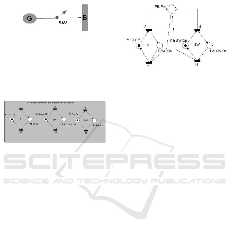
Figure 4: Single-Line Diagram of Electric Power System.
Petri net model of each elements that electric power
system is shown in the Figure 5.
it is observed that the bus will be energized if the
SW switch is closed and the generator is turned on.
In this way, a monitor will be synthesized so that it
can verify the instants in which the bus is energized.
From the Petri net shown in Figure 5, extract the inci-
dence matrix of the switch(SW)-generator(G) set and
the vector L.
Figure 5: PN Model of The Single-Line Diagram.
The bus will then be energized if the places p
2
and
p
4
are marked, that is, M(p
2
) + M(p
4
) = 2 is equiva-
lent to the vector L = [0 1 0 1]. the incidence matrix
and the calculation of the monitor will be.
B =



−1 1 0 0
1 −1 0 0
0 0 −1 1
0 0 1 −1



Using the Equation 15 it is determined that:
CB = LB =

1 −1 1 −1

CB is then the connections of the external place(the
monitor) with the transitions of the Petri net as shown
in Figure 6. The initial mark of the monitored
places is the same as the mark of the monitor, see
Equation(10). Therefore, the monitor place p
m
will
have zero marks initially for the example developed.
Whenever the place p
5
has two marks its mean the
bus is energized. Bus monitoring is shown in Figure
6
2.4 Modeling Electric Power System
Operation using Petri Net
The objectives of the control actions depend on the
point of operation of the electric power system. Un-
der normal conditions, the purpose of the control is to
Figure 6: Bus Monitoring.
keep the systems operating as efficiently as possible,
with voltage and frequency values close to the nomi-
nal (T. et al., 2020). On the other hand, when abnor-
mal conditions are verified, new objectives must be
pursued to restore the system to its normal operating
conditions, as soon as possible.
Control of the operation of an EPS consists of
commanding the components of interruption of the
system, to keep it under normal conditions, guaran-
teeing the safety and quality of the energy supplied.
2.4.1 Supervisory Control Theory using Petri
Nets Applied to EPS Operation
From this point on, the Petri Net is no longer au-
tonomous and becomes controllable, that is, the tran-
sitions now also depend, for their firing, on the exter-
nal places connected to transitions. The Equation(16)
shows how computing a controller.
]M + ]M
c
= K (16)
The marking can be rewrite as the following
(L +C)M = K (17)
substituting M by Petri Net Dynamic Equation, M =
M
o
+ Bq in the Equation(17) and rewiriting it, the fi-
nal result is shown in the Equation(19). The Equa-
tion(16) allows calculate the initial mark value of the
controller.


L
.. .
C


B
+
−


L
.. .
C


B
−
= 0 (18)
CB
+
−CB
−
= −LB
+
+ LB
−
In this way, Equation(19) provides the weight and di-
rections of the arcs that connect the controller to the
transitions of the original Petri net
CB = −LB (19)
The expanded Petri net N
h
has a marking M
(m+1)×1
h
such that preserves its marking by a T transformation,
T M =⇒ M
h
.
ICINCO 2022 - 19th International Conference on Informatics in Control, Automation and Robotics
662

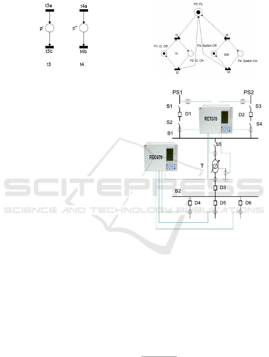
Figure 7: Equivalent PN to transitions.
Example: Now in the Figure 4 is desired to con-
trol the opening/closing of SW switch. Opening and
closing operation of SW is not allowed when the gen-
erator(G) is in On state. The controller must establish
restrictions on the free behavior of the Petri net mod-
els of the G generator and SW switch to not allow
those. The PN models free behavior of G and SW are
the same as shown in Figure 5. To restrict the states
reached from the Petri net the following equations can
be used:
p
2
+t
4
= 1
and
p
2
+t
3
= 1
Adding the two equations will find
2p
2
+t
3
+t
4
= 2
The restriction found has two transitions (events) and
a place (state). This situation eliminates the ability
to operationalize terms with different meanings. The
way to be able to operationalize this equation is to
transform one of the terms into others. Thus, can
convert the transitions of the equation by associat-
ing them with places or places associated with tran-
sitions. Figure 7 shows a way to associate transitions
with place. That way, rewriting the restriction find:
2p
2
+ p
0
+ p
00
= 2
So using the change and the Equations(19) and
(16) is founded:
CB = [+1, −1,±1, ±1]
and
m
c
= 1
The Figure 8 shows the expanded PN with the
controller p
c
. In this figure, it is observed the con-
troller with a mark releases the SW switch model al-
lowing to change marking. This occurs while the gen-
erator PN model is in the off state. When the model
of the generator goes into the On state (p
4
with mark)
the controller will lose the mark inhibiting the model
of the SW switch to change their states.
Figure 8: PN: Opening/Closing Controller Operation.
Figure 9: Bus Feeder System and Power Supply (Ltd,
2010).
3 APPLICATION IN
SUBSTATIONS
As an application, it is made the modeling, monitor-
ing and control of the EPS represented in Figure 9 by
its single line diagram. It is a substation composed
of two buses, [B
1
and B
2
], six circuit breakers [D
1
,
D
2
,·· · ,D
6
], five disconnect switches [S
1
,·· ·, S
5
], one
transformer and three energy consumers.
First of all, considering the substation de-
energized [i.e. the disconnect switches and circuit-
breaker assemblies are all disconnected or open].
With this, the following procedure
1
can be proposed
1
Any procedure proposed must be in agreement with lo-
cal standards and aligned with the concessionary that holds
the formal authorization to distribute electricity in the re-
Power System Operation Modeling, Monitoring and Control using Petri Nets
663

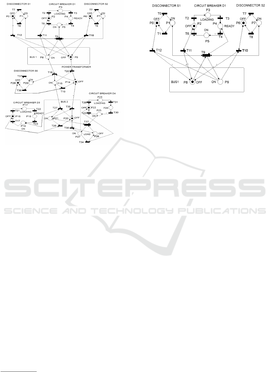
Figure 10: Substation Free Behaviour PN Modeling.
to energize the buses B
1
and B
2
:
1. To power on the Bus B
1
via PS
1
, must be given
priority to close the disconnecting switches S
1
and
S
2
and after these the circuit breaker D
1
must be
closed;
2. To power on the Bus B
1
via PS
2
, must given pri-
ority to close the disconnecting switches S
3
and
S
4
and after these the circuit breaker D
2
must be
closed;
3. To power on the Transformer T after the Bus B
1
is on, it must be given priority to close the discon-
nect switch S
5
. So after that, the circuit breaker D
3
can be closed and consequently the bus B
2
will be
on;
4. To energize some electric loads after bus B
2
is on,
one circuit breaker must switch on D
4
to D
6
with-
out setting an order of priority;
5. The procedure for shutdown the substation must
obey an inverse prioritization order those done for
startup it [i.e. first of all, it must disconnect the
loads by switching off D
4
to D
6
, then isolating
the bus B
2
through D
3
, following with the de-
energizing of the transformer through S
5
and so
on];
gion where that the substation is installed.
Figure 11: PS
1
Free Behaviour PN Modeling.
3.1 Free Behavior Modeling for
Substation
Some specifications are adopted for modeling of the
substation as following. The disconnect switches
have two possible states: (i) the connected state; and
(ii) the disconnected state. The circuit breakers have
4 states: (i) the Off state; (ii) Carrying the Spring
State; (iii) ready to go Into Operation State; and the
On State. For this modeling, abnormal conditions of
the equipment are not considered [for instance, the
broken state]. The buses also are represented by two
states: (i) de-energized; and (ii) energized.
The presence of the token depicts the current state
of the equipment. For instance, considering a discon-
nector switch where P
1
is the state that symbolizes
when it is disconnected and P
2
the state representing
when it is connected, then if a token is in P
2
it repre-
sents that the disconnector switch is closed, otherwise
[token in P
1
] it is open.
In Figure 10, a summarized version of the free be-
havior for the substation presented in Figure 9 is pre-
sented. The substation Petri net model consists of an
input PS
1
composed of two disconnect switches S
1
and S
2
and a circuit breaker D
1
, followed by the rep-
resentation of the input bus B
1
. After this, there is
the model of the disconnect switch (S
5
), responsible
for energizing the primary winding of the transformer.
To the right side of S
5
model is the representation of
the possible states of the power transformer. In the
bottom of the Petri net, all of the other models are
presented: the model to the circuit breaker D
3
, the
output bus B
2
and the energizing circuit breaker of a
load D
4
.
ICINCO 2022 - 19th International Conference on Informatics in Control, Automation and Robotics
664

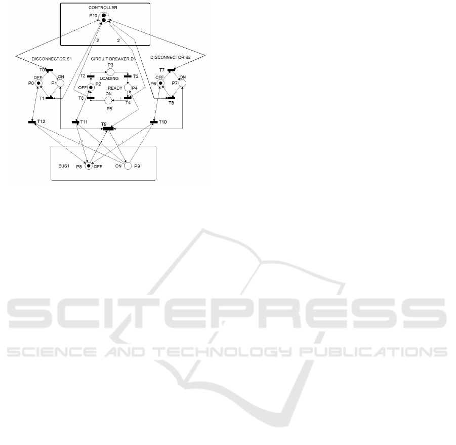
Figure 12: PS
1
System Control PN Modeling.
3.2 Controller Design for Sequence
Operation
In Figure 11 is shown the Petri net model of the
free behavior for the input PS
1
energizing the bus
B
1
. This representation does not contemplate the re-
strictions for the operation of the disconnect switches
and circuit breakers that affect the safe energization
or shutdown of the bus B
1
. These constraints are in-
timately related to the constructive aspects of these
operational control elements. For example, the ma-
nipulation of the disconnect switches must not be car-
ried out with the circuit-breaker switched on. Thus,
the correct way to energize the bus B
1
is closing the
disconnect switches S
1
and S
2
and after that close the
circuit breaker D
1
.
For the energizing and de-energizing operation of
the PS
1
, it is necessary to compute a controller that
can restrict some actions of the free behavior model.
For this, it is necessary to specify the controller ac-
tions to guarantee the correct sequence of events fir-
ing. A control system is presented in Figure 12. The
control specifications are represented by a set of linear
equations where their variables represent the marking
of the controlled places. The constant on the other
side of the equation will mean that the controlled
places will form a place invariant with the controllers
[see Equation(16)].
To specify the controllers, it is necessary to find
the incidence matrix B
c
of these places and also their
initial marking M
c0
. The incidence matrix B
c
is ob-
tained from both the control specifications and the in-
cidence matrix of the original petri net.
From Figure 12, the constraints on this feeder can
be found by making the following considerations with
respect to feeder free behavior model PS
1
:
1. If the current state of the circuit-breaker is closed
[i.e., P
5
with marks], it forces that the current
states of the disconnect switches are also on states
[P
1
and P
7
];
2. Generating equation P
5
+ P
1
+ P
7
= 3;
3. If the current state of one of the connect switches
is opened [i.e., P
0
or P
6
with marks] the breaker
can not to close [P
5
= 0];
4. Generating equation P
5
+ P
0
+ P
6
= 1;
Adding the two equations above one can get
2P
5
+ P
0
+ P
1
+ P
6
+ P
7
= 4
and consequently
L = [1, 1,0, 0,0, 2,1, 1,0, 0].
With L and the incidence matrix, the weights of
the arc that interconnects the controller with the tran-
sitions of the original Petri net are obtained from
C B = −L B = [±1, ±1,0, 0, −2,2, ±1,±1, 0,0].
The determination of the initial marking of the
controller is obtained through Equation(16). With the
value of the initial marking of the controlled places
[i.e., P
0
, P
1
, P
5
, P
6
and P
7
], the vector L and the con-
stant K, K = 4. Found: M
c0
= 2. With this informa-
tion the Petri net of Figure 12 is drawn.
The terms represented by ± correspond to the
nonzero position in the vector L that resulted in zero
in the calculation of Equation(19). In the formation
of the controlled Petri net, these positions will be
represented by autoloop. see Figure 12. The au-
toloop present between the transitions of the connect
switches models and the controller allows these tran-
sitions to fire without changing the controller mark-
ing. This condition releases the models of the connect
switches to move from the off state (P
0
and P
7
with to-
kens) to on state (P
1
and P
8
with tokens) freely. When
the model representing the circuit breaker goes to the
on state (P
5
with mark), the T
4
transition removes two
marks from controller (P
10
). The controller place, P
10
,
without marking inhibits firing of the transitions be-
longing to the switch models (T
0
, T
1
, T
7
, and T
8
). This
condition (P
10
without tokens) keeps the model of the
disconnect switches in the state that were before the
T
4
transition firing.
In agreement with the constraints imposed to de-
termine the controller, the following sequence of
events are possible: T
0
T
7
T
2
T
3
T
4
representing the on
states of the switches, breaker and bus(P
1
,P
5
,P
7
and
P
9
with marks) and another sequences are T
5
T
1
T
8
or T
5
T
8
T
1
representing the states off the disconnect
switches, circuit breaker and bus (M
0
). In relation
to the bus, it already loses the on status as soon as
Power System Operation Modeling, Monitoring and Control using Petri Nets
665

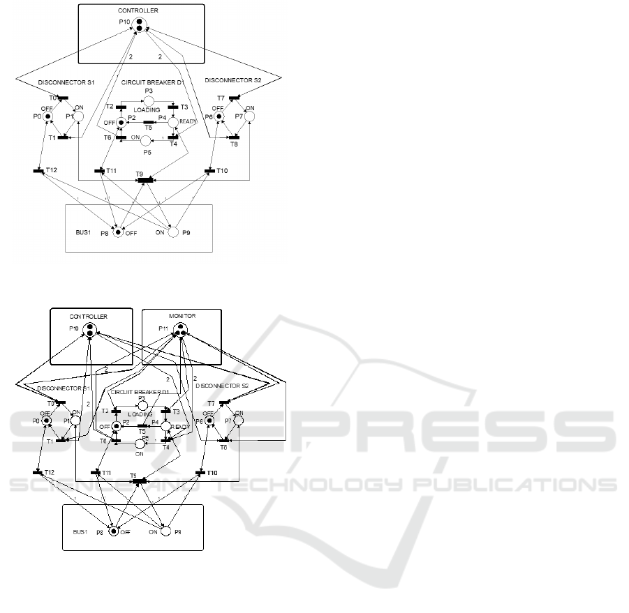
Figure 13: PN Model for PS1 with Uncontrolled and Ob-
servable Transition.
Figure 14: Structure of a monitor for PS1 with Failure Tran-
sition.
T
5
fires since the model contemplates the way the
switches and circuit breakers are physically intercon-
nected(series association).
3.3 Development of the Monitor
In figure 10 is shown the Petri net model for the in-
put power supply PS 1 of the sub-station presented
in Figure 6. A new transition T
5
has been inserted
to represent a failure event. This event connects both
the place that represents the Ready Circuit Breaker
status and the place that represents off State Circuit
Breaker Status. Thus, T
5
emulates possible problems
that may appear on the circuit breaker, such as loss of
elastic characteristics of the spring assembly, jammed
or worn contacts, etc. Consider T
5
be uncontrollable
and observable means that the controller can not in-
tervene in its firing but the monitor alarms if it comes
to fire.
So, given the Incidence matrix B of the Petri net of
Figure 13 and knowing that when specifying a moni-
tor for the main places those represents S
1
, S
2
and D
1
the vector L is will be.
L =

1 1 1 1 1 1 1 1 0 0 1

B =

















−1 1 0 0 0 0 0 0 0 0 0 0 0
1 −1 0 0 0 0 0 0 0 0 0 0 0
0 0 −1 0 0 1 0 0 0 0 0 0 1
0 0 1 −1 0 0 0 0 0 0 0 0 0
0 0 0 1 −1 0 0 0 0 0 0 0 0
0 0 0 0 1 −1 0 0 0 0 0 0 −1
0 0 0 0 0 0 −1 1 0 0 0 0 0
0 0 0 0 0 0 1 −1 0 0 0 0 0
0 0 0 0 0 0 0 0 −1 1 1 1 0
0 0 0 0 0 0 0 0 1 −1−1−1 0
0 0 0 0 −2 2 0 0 0 0 0 0 0

















And applying the condition for monitoring in the
Equation(15). It is determined that the weight of the
arches between the monitor place and the Perti net
will be:
B
m
=

±1±1±1±1−2 2 ±1 ±1±1±100±1

Transition T
5
is occupying the last column of the inci-
dence matrix B. It is a non-controllable transition and
therefore the monitor will not be able to intervene in
your fire. This condition eliminates in the computa-
tion of vector B
m
the arc that will link the place mon-
itor to the transition T
5
. That way, the monitor will
know if the transition T
5
has fired but it does not in-
terfere in your fire. The last field of the B
m
vector
loses the value -1 and retains the +1 value. See B
m
below.
B
m
=

±1±1±1±1−2 2 ±1 ±1±1±1001

The initial marking for the monitor will be ob-
tained through Equation(10). Thus, the new Petri net
is shown in Figure 14. By analyzing the Petri net of
Figure 14 are extracted the following informations:
1. The firing of all controllable transitions remains
invariant between the monitored and monitor
places.
2. The fire of the uncontrolled transition causes the
breaking of the invariant place, allowing the iden-
tification of the failure.
3. The number of monitor marks expresses the num-
ber of times the failure occurred.
4. The occurrence of the fault causes loss of control
by the controller P
10
.
5. The Monitor does not interfere in the actions of
the controller.
ICINCO 2022 - 19th International Conference on Informatics in Control, Automation and Robotics
666

4 CONCLUSIONS
In this work, the modeling framework of an EPS us-
ing Petri nets Place-Transition was adopted to analyze
issues relevant to monitoring and control in the op-
eration of an EPS. In the development of the model,
a linear transformation was used, which allows for-
mally solving monitoring and control problems. Us-
ing Linear Algebra techniques, an equation was de-
veloped that for boundary conditions, formalizes such
techniques. For monitoring analysis, the conservation
of the number of marks in the extended Petri net was
ensured, which leads the expanded Petri net to main-
tain the balance between the input and output inci-
dence matrix of the original Petri net, thus ensuring
the ownership of place invariants. As for the control
of the operation, it was established that the marking of
the extended Petri net is kept constant, which leads to
an incidence matrix of the expanded part as opposed
to the incidence matrix of the places to be controlled.
The work is completed with an application study that
was carried out using an electrical power system sub-
station. The selection of the places to be monitored
is made from a line vector, L vector, whose non-null
elements point to their positions. The product of this
vector with the incidence matrix of the original Petri
net generates the incidence matrix of the expansion
of the Petri net. This result determines the weight, the
direction of the arc and which events of the original
Petri net will link the Monitor or Controller place.
ACKNOWLEDGMENTS
This work was partially supported by CAPES
(Coordenac¸
˜
ao de Aperfeic¸oamento de Pessoal de
N
´
ıvel Superior).
REFERENCES
Amini, S., Pasqualetti, F., Abbaszadeh, M., and Mohsenian-
Rad, H. (2019). Hierarchical location identification of
destabilizing faults and attacks in power systems: A
frequency-domain approach. IEEE Transactions on
Smart Grid, 10(2):2036–2045.
Bin, S. Y., Ping, C. Y., and Zhan, B. (2015). Fault diagnosis
for power system using time sequence fuzzy Petri net.
In 3rd International Conference on Mechanical Engi-
neering and Intelligent Systems (ICMEIS), volume 1,
pages 729–735.
Cassandras, C. G. and Lafortune, S. (2009). Introduction to
discrete event systems. Springer Science & Business
Media.
David, R. and Alla, H. (1994). Petri nets for modeling of
dynamic systems - a survey. Automatica, 30(2):175–
202.
Dideban, A. and Alla, H. (2009). Feedback control logic
synthesis for non safe Petri nets. IFAC Proceedings
Volumes, 42(4):942 – 947.
Fendri, D. and Chaabene, M. (2019). Hybrid Petri net
scheduling model of household appliances for optimal
renewable energy dispatching. Sustainable Cities and
Society, 45:151 – 158.
Giua, A. (1992). Petri Nets as Discrete Event Models for
Supervisory Controls. PhD thesis, Dept. Electrical
Computer and Systems Engineering, Rensselaer Poly-
technic Institute.
Holloway, L. E., Guan, X., and Zhang, L. (1996). A gen-
eralization of state avoidance policies for controlled
Petri nets. IEEE Transactions on Automatic Control,
41(6):804–816.
Komenda, J., Lahaye, S., Boimond, J.-L., and van den
Boom, T. (2018). Max-plus algebra in the history of
discrete event systems. Annual Reviews in Control,
45.
Krogh, B. H. and Holloway, L. E. (1991). Synthesis of feed-
back control logic for discrete manufacturing systems.
Automatica, 27(4):641–651.
Lin, W., Luo, J., Zhou, J., Huang, Y., and Zhou, M. (2016).
Scheduling and control of batch chemical processes
with timed Petri nets. In IEEE International Confer-
ence on Automation Science and Engineering (CASE),
pages 421–426.
Ltd, A. (2010). Abb special report iec 61850. Technical
report.
Murata, T. (1989). Petri nets: Properties, analysis and ap-
plications. Proceedings of IEEE, 77(4):541–580.
Papadopoulos, C. T., Li, J., and O’Kelly, M. E. J. (2019).
A classification and review of timed markov models
of manufacturing systems. Computers and Industrial
Engineering, 128:219 – 244.
Souza, M., Lima, E., and Cerqueira, J. (2016). Electric
power system operation: A Petri net approach for
modelling and control. In 13th International Con-
ference on Informatics in Control, Automation and
Robotics, volume 1, pages 477 – 483.
T., S., Vieira, G. G., Salles, M. B., and Avila, S. L. (2020). A
trip-ahead strategy for optimal energy dispatch in ship
power systems. Electric Power Systems Research,
page 106917.
Tekiner-Mogulkoc, H., Coit, D. W., and Felder, F. A.
(2012). Electric power system generation expansion
plans considering the impact of smart grid technolo-
gies. International Journal of Electrical Power & En-
ergy Systems, 42(1):229 – 239.
Weiss, T. and Schulz, D. (2015). A generic optimiza-
tion tool for power plant dispatch and energy storage
system operation. In 50th International Universities
Power Engineering Conference (UPEC), pages 1–6.
Wu, X., Tian, S., and Zhang, L. (2019). The internet
of things enabled shop floor scheduling and process
control method based on Petri nets. IEEE Access,
7:27432–27442.
Power System Operation Modeling, Monitoring and Control using Petri Nets
667