Using Convolutional Neural Networks for Detecting Acrylamide in

Biscuit Manufacturing Process

Dilruba Topcuoglu

, Berat Utkan Mentes

, Nur Askin

, Ayse Damla Sengul

, Zeynep Deniz Cankut

Talip Akdemir

, Murat Ayvaz

, Elif Kurt

, Ozge Erdohan

, Tumay Temiz

and Murat Ceylan

Advanced Analytics Solutions, Most Technology/Yıldız Holding, Istanbul, Turkey

Northstar Innovation, Yıldız Holding, Istanbul, Turkey

Department of Electrical-Electronics Engineering, Konya Technical University, Konya, Turkey

Keywords: Acrylamide, Deep Learning, Image Processing, CNN Algorithm.

Abstract: Based on a research in 2002 (Ozkaynak & Ova, 2006), acrylamide substance is formed when excessive heat

treatment (e.g. frying, grilling, baking) is applied to starch-containing products. This substance contains

carcinogenic and neurotoxicological risks for human health. The acrylamide levels are controlled by random

laboratory sampling. This control processes which are executed by humans, cause a prolonged and error prone

process. In this study, we offer a Convolutional Neural Network (CNN) model, which provides acceptable

precision and recall rates for detecting acrylamide in biscuit manufacturing process.

1 INTRODUCTION

In the food industry, the acrylamide substance can be

found in the final products due to the exposure of

carbohydrate-containing foods to excessive heat

(Ozkaynak

& Ova, 2006). This substance is

understood to have carcinogenic effects on humans;

therefore, it must not be consumed.

Providing healthier products to our customers and

maintaining their trust is vital. The solution we

designed guarantees us that every product that we will

be producing is under control and they can be safely

consumed. This way, production efficiency can be

maintained in terms of time, waste and cost.

Before developing our solution, the initial

solution method was twofold:

1. Random sample parties are selected from the

products to detect the number of products

containing acrylamide levels two times a year

2. Eye control to detect color change is executed

during production.

We collected the product photos that contains

acrylamide above and belove the accepted levels to

build a dataset. Normalization and resizing operations

are also planned to be used to make this data set

suitable in the future. After creating the dataset, data

manipulation is performed by changing brightness,

rotation, scrolling, etc. We shaped the model by

optimizing the parameters to provide better

recognition accuracy. We performed data

augmentation by using the model features. After we

created enough data for the model to learn, we started

to build our model. After training the model with the

data that we split into train and test partitions, we

tested our model in the quality control process.

By solving our problem using the image

processing method, we eliminated the risk of

overlooking inefficiency by avoiding manual control.

Control process is also automated by using the

cameras. Since it is not controlled by people, the

speed of the production line is also increased. This

algorithm can be used for the quality control

processes of other products or to measure the amount

of acrylamide levels in similar products.

2 MATERIAL AND METHODS

Detection of acrylamide is one of the most

considerable problem for each company producing

carbohydrate-containing foods. Therefore, the

solution to this problem is also important. By

referencing the literature, we tried to develop a

solution to determine acrylamide in consumed foods

by using different methods.

In the model that is used to detect acrylamide in

potato chips, BatchNormalization() is used to prevent

500

Topcuoglu, D., Mentes, B., Askin, N., Sengul, A., Cankut, Z., Akdemir, T., Ayvaz, M., Kurt, E., Erdohan, O., Temiz, T. and Ceylan, M.

Using Convolutional Neural Networks for Detecting Acrylamide in Biscuit Manufacturing Process.

DOI: 10.5220/0011310100003269

In Proceedings of the 11th International Conference on Data Science, Technology and Applications (DATA 2022), pages 500-503

ISBN: 978-989-758-583-8; ISSN: 2184-285X

the model from overfitting. This function, brings high

success to prevent overfitting in image processing,

also provided successful results here. For this reason,

we used BatchNormalization() to suppress overfitting

in our model. Moreover, U-Net was used to classify

images of potato chips. The data we used in our model

was split as train, validation and test. Sigmoid is one

of the suitable function as activation for the output

layer of the model; since, it returns a value between 0

& 1. Another process is the normalization step of the

data set. Due to the data volume, algorithm execution

time should also be considered. For this reason, we

arranged the photos by the highest number of pixels

(255). Thus we made them more comfortable to

process in the [0,1] range. In the article (Maurya et

al., 2021), the transfer learning method is used while

constructing the model. Transfer learning is a

machine learning methodology that focuses on

storing the knowledge gained while solving a

problem and applying it to another similar problem

(Yiğit

& Yeğin, 2020). We wanted to use unique

methods in our model to stay flexible to dynamic

business requirements, so we did not choose to use

pre-trained models.

The article (Arora, M. & Mangipudi, P. & Dutta,

M. K. 2020)

studied the amount of acrylamide in

potato chips, which is the study (Maurya et al., 2021),

also investigated. In this approach, they used a pre-

trained model and obtained a high model accuracy.

In this article, Acrylamide is detected in potato

chips with the help of LC-MS Analysis. Liquid

Chromatography with Tandem Mass Spectrometry

(LC-MS-MS) is a powerful analytical technique that

combines the separating power of liquid

chromatography with the highly sensitive and

selective mass analysis capability of triple quadrupole

mass spectrometry

(EAG Laboratories, n.d.) This

method is checking whether it contains acrylamide by

looking at the distribution of colors on the chips. We

did not try this method as it would not help in

accelerating our process in line with our targeted

outputs (Gökmen et al., 2007).

In this approach, they tried to reach the result with

the help of chemical studies. We did not use this

solution method here due to its distance from our

targets and work area (Alpözen et al., 2013).

In the light of the information obtained as a result

of the literature review, the Acrylamide substance

was not detected by image processing with the CNN

algorithms, which was specifically trained for

Acrylamide substance. Therefore, we wanted build

our own model architecture from scratch.

3 EXPERIMENTS

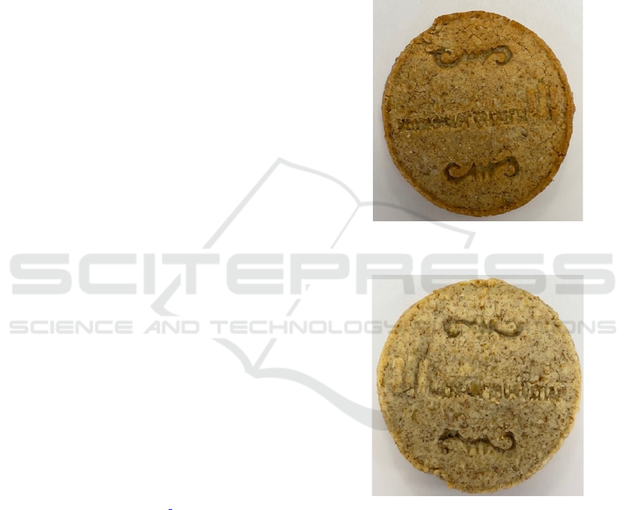
We collected and assorted the photos of the products

taken by the business unit. Overall, we have 572

pictures; 201 of them are above the threshold

(meaning they consist acrylamide greater than the

threshold), 371 of them are below the threshold

(meaning they do not consist acrylamide greater than

the thresholds) (see Figure 1 & 2).

Figure 1: A sample above the threshold (label as

acrylamide).

Figure 2: A sample below the threshold (label as non-

acrylamide).

We split our data set into test & train data sets; for

training we used 160 pictures and for testing we used

40 pictures from both above and below datasets. After

the split process, we set data to 224x280. We used this

data to train and test the Convolutional Neural

Network model.

Using Convolutional Neural Networks for Detecting Acrylamide in Biscuit Manufacturing Process

501

3.1 Creating the Model

There are five convolution layers in total in the

Convolutional Neural Network model that we

designed.

The kernel size of the first four layers was 3x3,

and the last layer's kernel was 1x1. After each

convolution layer, there was a Batch Normalization

layer.

We spread an effort to reduce the data size.

Therefore, we used MaxPooling in size 2x2 after the

first four convolutional layers. After the last

convolution layer, we transformed the data into one-

dimensional tensor by flattening. This one-

dimensional tensor was given as an input to the fully

connected layers.

Our model had six fully connected layers. The

first five fully connected layers contain 128, 64, 32,

16, 10 neurons, and the fully connected output layer

contains 1 neuron.

To prevent over-fitting, dropout layers were used

after convolution and fully connected layers.

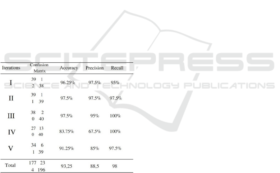
For the cross-validation method, we created 5

different data partitions by dividing the data into

random groups. All groups were set to contain an

equal amount of data. We used 80% of the data for

training and 20% for testing. Batch Size was set to 1

to allow more accurate gradient value calculation and

to reduce linearity.

We trained the Convolutional Neural Network

model with Adam optimizer at 100 epochs and set the

initial learning rate to 0.0001.

The loss function was chosen as the binary cross-

entropy, which provided the best binary classification

result.

After training the model, we sent the test data to

the model and classified the predicted label value by

comparing it with the values found as a result of the

sigmoid function.

All operations were executed on NVIDIA

GeForce GTX 1080 Ti workstation with 64GB RAM.

Rescaled using MATLAB 2020b, classification was

performed using Python 3.9.7 and Keras 2.8.0 (using

Tensorflow 2.8.0 backend).

3.2 Data Augmentation

Since the data set we have was not enough for the

model to learn completely, the data was replicated

with the help of the ImageDataGenerator() function.

In this step, our train and test data;

• By specifying the rotation_range parameter,

which rotates the image randomly clockwise

by the given degree (40 degrees),

• By specifying the rescale parameter 1./255,

which performs the normalization process,

• By specifying the zoom_range parameter 0.2,

which is used to zoom the image,

• By specifying the shear_range parameter 0.2,

which distorts the image in the axis direction,

• To move the image horizontally, by specifying

the width_shift_range parameter to 0.2,

• To move the image vertically, by setting the

height_shift_range parameter to 0.2,

• Set the horizontal_flip parameter to True to

flip the image horizontally.

were multiplied. As a result, we obtained 5 new

pictures from each training picture. In the end, we had

800 pictures for both above and below threshold

classes.

After reshaping the dimensions of our data, the

learning process was carried out by fitting our model.

We calculated our success metric "accuracy" which is

the number of correct predictions/total number of

predictions. Although accuracy was our main

evaluation metric, evaluating it alone was not the

right approach. We also used Precision and Recall

metrics to better observe the reliability of Accuracy.

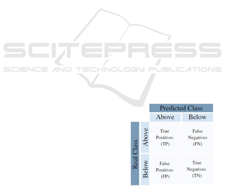
The precision tells us how many of the positively

predicted class predictions are essentially positive. In

other words, it refers to the formula TP/(TP+FP).

Recall, on the other hand, gives the ratio of how many

of the transactions we need to predict positively are

essentially positively predicted. In other words, it is

formulated as TP / (TP+FN). When we took the

average of 5 results, we got 93.25% Accuracy, 88.5%

Precision, 98% Recall.

Figure 3: Confusion Matrix Representation.

DATA 2022 - 11th International Conference on Data Science, Technology and Applications

502

4 CONCLUSIONS

We predicted the acrylamide levels as belove or

above threshold) in our production lane by using

image processing with a Convolutional Neural

Network model that was specifically built for

detecting Acrylamide substances. The results

obtained are summarized below.

• Our products can be delivered to consumers

with high confidence,

• The old way of detecting acrylamide in the

product will not be needed,

• Thus, the product line will progress faster

• Packaging of the products will be faster,

• The risk of detection errors will be reduced as

it switches from human control to machine

control

• In the future, we are planning to integrate our

model into a mobile application to make our

solution user friendly.

Table 1: Classification results for five-fold cross-validation

using the Convolutional Neural Network model and the

total result obtained by adding the folds.

ACKNOWLEDGMENTS

In Figure 3 Expressed in this way, "above" stands for

Positive, "below" stands for Negative.

REFERENCES

Alpözen, E. & Güven, G. & Üren, A. (2013) –

Determination of Acrylamide Levels of Light Biscuit

by LS-MS/MS. Akademik Gıda 11(3-4)

Arora, M. & Mangipudi, P. & Dutta, M. K. (2020) - Deep

Learning neural networks for acrylamide identification

in potato chips using transfer learning approach.

Journal of Ambient Intelligence and Humanized

Computing

EAG Laboratories (n.d.), Liquid Chromatography -

Tandem Mass Spectrometry (LC-MS-MS), Retrieved

from June 2022, https://www.eag.com/techniques/

mass-spec/lc-ms-ms/

Gökmen, V. & Şenyuva, H.Z. & Dülek B. & Çetin, A.E.

(2007) – Computer Vision-based image analysis for the

estimation of acrylamide concentrations of potato chips

and French fries. Food Chemistry 101

Maurya, R. & Singh, S. & Pathak, V. K. & Dutta, M. K.

(2021) – Computer‐aided automatic detection of

acrylamide in deep‐fried carbohydrate‐rich food items

using deep learning: Machine Vision and Applications,

32 : 79

Ozkaynak, E. & Ova G. (2006), Akrilamid Gıdalarda

Oluşan Önemli bir Kontaminant – 1: Akrilamid Gida

Dergisi - Dergipark, 4:3

Yiğit, G. & Yeğin M. N. (2020) – Öğrenme Aktarımı/

Transfer Learning (Nova Research Lab)

Using Convolutional Neural Networks for Detecting Acrylamide in Biscuit Manufacturing Process

503