Nonlinear Set-based Model Predictive Control for Exploration:

Application to Environmental Missions

A. Anderson

1,2 a

, J. G. Martin

3 b

, N. Bouraqadi

1 c

, L. Etienne

1 d

, K. Langueh

1 e

L. Rajaoarisoa

1 f

, G. Lozenguez

1 g

, L. Fabresse

1 h

, J. M. Maestre

3 i

and E. Duviella

1 j

IMT Nord Europe, Institut Mines-T

ecom, Centre for Digital Systems, F-59000 Lille, France

Instituto de Desarrollo Tecnol

ogico para la Industria Qu

ımica (INTEC),

Consejo Nacional de Investigaciones Cient

ıﬁcas y Tecnicas (CONICET), Santa Fe, Argentina

Departamento de Ingenier

ıa de Sistemas y Autom

atica, Universidad de Sevilla,

C/ Camino de los Descubrimientos, s/n., 41092 Sevilla, Spain

Keywords:

Nonlinear MPC, Unmanned Vehicles, Environmental Missions, Water Quality Assessment.

Abstract:

Acquiring vast and reliable data of physicochemical parameters is critical to environment monitoring. In the

context of water quality analysis, data collection solutions have to overcome challenges related to the scale of

environments to be explored. Sites to monitor can be large or remote. These challenges can be approached by

the use of Unmanned Vehicles (UVs). Robots provide both ﬂexibility on intervention plans and technological

methods for real-time data acquisition. Being autonomous, UVs can explore areas difﬁcult to access or far

from the shore. This paper presents a nonlinear Model Predictive Control (MPC) for UV-based exploration.

The strategy aims to improve the data collection of physicochemical parameters with the use of an Unmanned

Surface Vehicle (USV) targeting water quality analysis. We have performed simulations based on real ﬁeld

experiments with a SPYBOAT® on the Heron Lake in Villeneuve d’Ascq, France. Numerical results suggest

that the proposed strategy outperforms the schedule of mission planning and exploration for large areas.

1 INTRODUCTION

The problem that we consider is that of explo-

ration missions, which implies both mission planning

and design of autonomous control strategies Nigam

(2014). Exploration requires ofﬂine and online mo-

tion planning, i.e., a sequence of connected linear

tracks covering the entire region to explore. In Go-

erzen et al. (2010) a complete overview of the existing

motion planning algorithms is provided. In case the

motion planning is solved ofﬂine, the parameterized

reference allows the USVs to navigate several desired

https://orcid.org/0000-0001-6626-500X

https://orcid.org/0000-0002-0362-5554

https://orcid.org/0000-0001-6459-4934

https://orcid.org/0000-0003-0931-843X

https://orcid.org/0000-0002-5984-2187

https://orcid.org/0000-0001-9624-5843

https://orcid.org/0000-0001-6875-7702

https://orcid.org/0000-0002-2223-7258

https://orcid.org/0000-0002-6343-5445

https://orcid.org/0000-0002-1622-0994

regions by an autonomous control strategy. A pop-

ular control technique of growing successes, particu-

larly in the ﬁeld of MPC, is the path-following prob-

lem. A thorough review of Nonlinear MPC trajectory

tracking and path-following controllers with applica-

tion to nonholonomic robots can be found on Nasci-

mento and Saska (2019). On the other hand, for ex-

ploration missions performed by multitarget tracking,

there are several control designs adapted for speciﬁc

environments to provide an energy efﬁcient and ro-

bust solution. For instance, Sarunic and Evans (2014)

provides a hierarchical MPC that enables an efﬁcient

trajectory for the UAVs; a nonlinear MPC scheme for

navigation for constrained enviroment is proposed in

Lindqvist et al. (2020); Prodan et al. (2013) (the last

paper provide a path design via differential ﬂatness);

Bertrand et al. (2014) presents a framework for the co-

operative guidance of a ﬂeet of autonomous vehicles

with optimal trajectories obtained for an exploration

mission on a grid zone. A full discussion about the

general relation between different control objectives,

covering set-point stabilization, trajectory tracking,

path-following and their approaches within the non-

230

Anderson, A., Martin, J., Bouraqadi, N., Etienne, L., Langueh, K., Rajaoarisoa, L., Lozenguez, G., Fabresse, L., Maestre, J. and Duviella, E.

Nonlinear Set-based Model Predictive Control for Exploration: Application to Environmental Missions.

DOI: 10.5220/0011307300003271

In Proceedings of the 19th International Conference on Informatics in Control, Automation and Robotics (ICINCO 2022), pages 230-237

ISBN: 978-989-758-585-2; ISSN: 2184-2809

linear MPC framework are included in Matschek et al.

(2019). Although interesting, the aforementioned

works and the most literature on MPC for exploration

are based on set-point stabilization and the beneﬁts

of the set-based MPC (i.e., general invariant set sta-

bilization) on the exploration missions have not been

explore.

The stabilization of target sets instead of single

points is more suitable in cases where it is enough to

reach at least one state inside a target region. Such is

the case of water resource management, where the ex-

ploration mission usually aims to cover large surface

of water with an USV to visit regions where a mea-

surement needs to be acquired Anderson et al. (2022).

In this scenario, the properties of invariant sets are

useful to provide robustness, ﬂexibility, extension of

the domain of attraction, between other beneﬁts. The

set stabilization can be framed in the context of set-

based MPC Blanchini and Miani (2015); Anderson

et al. (2018) where a general invariant set is consid-

ered as a control objective.

In this context, the main contribution of this article

is to present a novel set-based MPC formulation for

nonlinear systems for exploration large areas with an

USV. The proposal is based on a set of meshing of the

region to be explored with a twofold aims, to conﬁg-

ure a simple motion planning ofﬂine for the problem

and to use the sets composing the meshing as target

sets for the controller. Several simulation results tar-

getting water quality assessment show the properties

of the proposed controller.

1.1 Notation

We denote with N the sets of integers, N

:= N ∪ {0}

and I

:= {0, 1,.. .,i}. The ceiling function is deﬁned

by ceil(x) := min{n ∈ N : x ≤ n}. Consider two sets

U ⊂ R

and V ⊂ R

, containing the origin and a real

number λ. The Minkowski sum U ⊕ V ⊂ R

is de-

ﬁned by U ⊕ V = {(u + v) : u ∈ U, v ∈ V }; the set

U \ V ⊂ R

is deﬁned as U \ V = {u : u ∈ U ∧ u 6=

V }; and the set λU = {λu : u ∈ U} is a scaled set of

U. The close ball with center in x ∈ R

and radius

ε > 0 is given by B(x,ε) := {y ∈ R

: kx − yk ≤ ε}.

The point x is an interior point of U if the there exists

ε > 0 such that the open ball B(x,ε) ⊆ U. The inte-

rior of a set U is the set of all its interior points and it

is denoted by intU.

2 NONLINEAR SYSTEM AND

PRELIMINARY ANALYSIS

The dynamic process discussed in this work con-

sists in the class of discrete-time nonlinear system de-

scribed by the following equations

(

x(i + 1) = f (x(i),u(i)),

x(0) = x

(1)

where x(i) ∈ X ⊂ R

represents the measured states

of the system and u(i) ∈ U ⊂ R

the control input

at time i. The constraint sets X and U are compact

and convex with the origin inside, and the function

f : X × U → X is continuous with f (0, 0) = 0.

The following deﬁnition presents the concept of

invariance sets of control.

Deﬁnition 1 (Control Invariant Set - CIS). The set

Ω ⊂ X is a control invariant set (CIS) for system (1) if

for all x ∈ Ω there exists u ∈ U such that f (x, u) ∈ Ω.

The CIS has an associated corresponding input set

given by

Ψ(Ω) := {u ∈ U : ∃ x ∈ Ω such that f (x, u) ∈ Ω},

meaning that every input on Ψ(Ω) leaves at least one

state of Ω inside Ω.

A CIS is called a Contractive CIS if the condition

on Deﬁnition 1 is replaced by: for every x ∈ Ω there

is u ∈ U such that f (x,u) ∈ int Ω.

3 SET-BASED MPC

A generalization of the MPC controller for tracking

invariant sets is presented. The idea is to track and

reach sets that not only include stationary states, but

also transient states. We start with a quite general for-

mulation, that is particularized in the next subsections

to different applicable cases. Also consider the fol-

lowing deﬁnition.

Deﬁnition 2 (Generalized Distance Stage Cost Func-

tion). A generalized distance function d(x,Ω), from

x to the CIS Ω, is a function with the following prop-

erties: (1) d(x,Ω) is convex and continuous for all

x ∈ X, (2) d(x,Ω) = 0 for all x ∈ Ω, (3) d(x,Ω) > 0

for all x ∈ X \ Ω.

The proposed controller cost function will be

given by:

(x,Ω;u) =

N−1

∑

j=0

αd(x

,Ω) + βd(u

,Ψ(Ω)), (2)

Nonlinear Set-based Model Predictive Control for Exploration: Application to Environmental Missions

231

where α and β are positive real numbers, N is the

prediction horizon, the initial state x = x

, the pre-

dicted states x

j+1

= f (x

) and the input sequence

u = {u

,· · · ,u

N−1

Remark 3. The usual terminal cost associated with

the terminal predicted state x

can be omitted on Eq.

(2) if x

is force to belong to the set Ω, i.e., d(x

,Ω) =

0. As usual in MPC design, a local control action ¯u

that will act for predictions inside the terminal set Ω

will have also null cost since ¯u ∈ Ψ(U).

The general set-based MPC is given by the follow-

ing optimization problem solved at each sample time

k ∈ N.

min

(x,Ω;u) (3)

s.t. x

= x,

j+1

= f (x

), j ∈ I

N−1

∈ X, u

∈ U, j ∈ I

N−1

∈ Ω

Taking into account the receding horizon policy,

the control law at time k is given by the ﬁrst element

of the optimal sequence u

of the optimization prob-

lem given by (3) solved at time k.

Consider the next Lemma for the asymptotic sta-

bility of the closed-loop system.

Lemma 4. If Ω ⊂ X is a CIS for system (1) in the

cost function (2), then Ω is asymptotic stable for the

closed-loop system (1) controlled by the set-based

MPC given by (3).

Proof. The proof can be found on Blanchini and Mi-

ani (2015). It is stated that under the hypothesis of the

Lemma there is a Lyapunov function (given by the op-

timal cost V

(·)) that is a decreasing function on the

level sets of the generalized distance function used on

the function cost.

Next section presents an extension of the set-based

MPC to tracking multi-target sets.

3.1 Multi-target Tracking

Consider now that the closed-loop system has to reach

every element on the set

Ω = {Ω

,Ω

,· · · ,Ω

} with

Ω

⊂ X for i = 1, ··· ,K, in the speciﬁed order. This

is, once the controlled system reaches the target set

Ω

∈

Ω, the objective change to Ω

j+1

and so on un-

til the state of the system converge to Ω

. Clearly,

a condition must be establish in order to switch tar-

get every time the current target is reached. Here a

state-dependent MPC will be used to decide when a

target set is considered a reached set (according the

position of the current state). Consider the following

deﬁnition.

Deﬁnition 5 (Reached set). The ﬁrst set on

Ω, i.e.,

Ω

is considered a reached set if x(i) ∈ Ω

for some

i > 0. For k > 1, the target set Ω

∈

Ω is considered

a reached set if x(i) ∈ Ω

for some i > 0 and the pre-

vious sets Ω

,. . .,Ω

k−1

are reached sets.

As it can be seen, the condition for a set on

Ω to

be a reached set is deﬁned inductively.

The current target set, Ω

, which it depends on the

position of the current state x = x(i) is given by the

deﬁnition.

Deﬁnition 6 (Current target set). Given the sates of

the closed-loop system x(i) ∈ X for i = 0,. ..,k, where

x = x(k) is the current state at time k. The current

target set, Ω

, is given by

Ω

:= {Ω

k+1

: k = max{i : Ω

is a reached set}}

(4)

In the case that there is not reached sets then Ω

Ω

, for x = x(k), it deﬁnes the current objective on

time k.

The following MPC formulation to track sets is

based on the formulation presented on Limon et al.

(2005). The approach of this mentioned work was

to track sets with the aim of extends the domain of

attraction of the controller.

Considering the control law derived from solving

by the receding horizon strategy the following opti-

mization problem.

min

V (x,Ω

,u) (5)

s.t. x

= x,

j+1

= f (x

), j ∈ I

N−1

∈ X, u

∈ U, j ∈ I

N−1

∈ Ω

For an asymptotic stability condition consider the

next Lemma.

Lemma 7. If Ω

∈

Ω is a Contractive CIS for all j =

1,. . .,K, then every Ω

∈

Ω is a reached set for the

closed-loop system controlled by the MPC given on

(5).

Proof. If the current target set Ω

= Ω

is a Contrac-

tive CIS for system (1), the results proposed on An-

derson et al. (2018) proves that the closed-loop sys-

tem will reach in ﬁnite-time the set Ω

. Therefore,

according the formulation, once the target set Ω

reached, the current state switch to Ω

= Ω

j+1

. The

proof is concluded by induction.

ICINCO 2022 - 19th International Conference on Informatics in Control, Automation and Robotics

232

The following section provides the main result of

the paper. The proposal is an extension of the above

MPC formulation that aims to improve the perfor-

mance of the controlled trajectory.

4 PROPOSED MPC

In this section, the MPC based on sets for tracking

multi-target set is extended to improve performance.

To this end a dual-MPC is formulated, where the goal

of the ﬁrst mode is to reach only the current target

set Ω

= Ω

, by means of (5). The second mode is

activated when the current state x is close enough of

Ω

, this mode aims to give more importance to the

target set that became next, i.e., Ω

j+1

To trigger the second mode the current state must

be close enough of Ω

. This condition can be stated

by the inclusion of the current state on the fattening

set of Ω

Deﬁnition 8 (Fattening set). Let Ω

⊂ R

be the cur-

rent target set of control, and let ε > 0, we denote the

ε-fattening set of Ω

(Ω

)

:= ∪{B(x,ε) : x ∈ Ω

Remark 9. The term ’close enough’ of the current

target set is a parameter of the control design and can

be selected by chosen an appropriate ε.

The second mode is activated when the current

state is on (Ω

)

, at this time the design of the con-

trol consider the next target set, i.e. if Ω

= Ω

then

the next target set is Ω

j+1

. The following properly

deﬁnes the second target set, Ω

Deﬁne Ω

as in Eq. (4), and the set Ω

as follows:

Ω



Ω

j+1

, being Ω

= Ω

, x ∈ (Ω

)

Ω

, otherwise

(6)

Note that, if the current state x /∈ (Ω

)

, then it is

considered that Ω

= Ω

. This detail allows to for-

mulate the problem in a consistent way.

Consider now the function N

: X → I

that de-

ﬁnes the prediction horizon of the proposed con-

troller:



ceil(

Nd(x,Ω

)

), x ∈ (Ω

)

N, otherwise

Note that for the ﬁrst mode, i.e. when x /∈ (Ω

)

the prediction horizon is N. For the second mode, i.e.

when x ∈ (Ω

)

, the prediction horizon decreases with

the distance of the current state x to the current target

set. The ceil(·) function is considered for N

to be an

integer number.

Remark 10. Function N

is a decreasing function

with maximum value when x belongs to the bound-

ary of (Ω

)

, given by N

= N; and a minimum value

when x ∈ Ω

, given by N

= 0.

The second mode computes N

predictions to min-

imize the distance of the states to Ω

, and N −N

pre-

dictions to minimize the distance of the states to Ω

The cost function is given by

(x;u) =

−1

∑

j=0

Ω

) +

N−1

∑

j=N

Ω

) (7)

where `

Ω

) := αd(x

,Ω) + βd(u

,Ψ(Ω)),

and p,q > 0 are weight values.

The nonlinear MPC is given by the following op-

timization problem solved at each sample time i ∈ N.

min

(x;u) (8)

s.t. x

= x,

j+1

= f (x

), j ∈ I

N−1

∈ X, u

∈ U, j ∈ I

N−1

∈ Ω

The solution of Problem (8) is the optimal con-

trol sequence u

= {u

,· · · ,u

N−1

}. Taking into ac-

count the receding horizon policy, the control law at

time i is given by κ = u

(the ﬁrst element of the op-

timal control sequence), which is applied to the real

plant at every time step i.

4.1 Some Quantitative Properties of the

Proposal

In what follows, some numerical results are shown to

clarify the nontrivial properties of the proposed con-

troller.

We consider the USV model represented by Eq.

(9). With abuse of notation let deﬁne the current state

of the vessel by

x(i) = (x,y, ψ,u,v, r),

for every time i ≥ 0. Where x, y, z represent position

sates, on the surface (x,y) and ψ is the ’direction po-

sition’ of the vehicle in the inertial frame. Meanwhile

u,v, r represent the velocities states, i.e., surge (for-

ward), sway (perpendicular) and yaw (angular), re-

spectively.

The ﬁrst simulations attempts to show the an-

ticipatory behaviour of the proposed control. Con-

sider the paths given by

Ω = {Ω

,· · · ,Ω

} and

Ψ =

{Ψ

,· · · ,Ψ

} on the surface of the water (see Fig. 1).

This two paths are a reﬂection of each other.

Nonlinear Set-based Model Predictive Control for Exploration: Application to Environmental Missions

233

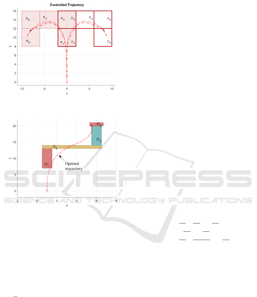
Figure 1: Two different controlled trajectories to follow

path

Ω and path

Ψ.

Figure 2: Optimal trajectory that pass over every target set

Ω

j = 1,. .., 4.

Note that both controlled trajectories of the vessel

are the same until the USV is ’close enough’ of the

ﬁrst target set in order to activate the second mode of

the control. At this point, both trajectories take dif-

ferent directions according the orientation of the path

that is followed. This anticipatory behaviour remains

until the vessel reaches the last target set on every

path.

Consider now the scenario presented on Fig. 2.

The objective is to drive the initial state x(0) =

(0,0,

,0, 0, 0) to Ω

, from there to Ω

then to Ω

and ﬁnally to Ω

. There are inﬁnite trajectories and

countless strategies to fulﬁll this objective, however

the optimal trajectory - given by proposed strategy -

selects the optimal position to pass through Ω

con-

sidering that from there the system need to be driven

to Ω

j+1

, for j = 1,. .., 3. It is noteworthy that the opti-

mal trajectory reaches only the boundary of Ω

, since

it is enough to reach the last target set Ω

from there.

5 SPYBOAT®’S DESCRIPTION

In this section the description of the USV used on the

simulation results and the real experiment described

on Section 6 is presented.

The CT2MC company has designed a range of

vessels dedicated to answer the need of data monitor-

ing of freshwater resource. The SPYBOAT® technol-

ogy follows standard equipment conﬁguration includ-

ing multiple sensors (localization system, compass,

sonar, camera) and is propelled by two independent

actuators. Thus the heading is controlled through a

differential thrust method.

The USV is equipped with a Hyperion optical sen-

sor from Valeport, for the measurement of the tur-

bidity. It is also equipped with Tripod sensors from

AquaLabo to measure the temperature, Dissolved

Oxygen, pH, and conductivity.

5.1 USV Nonlinear System

In Hervagault (2019) a kinematic model for the SPY-

BOAT® vessel was identiﬁed based following stan-

dard assumptions.

The marine craft moves on an horizontal plane and

only surge, sway and yaw are considered. The result-

ing is a nonlinear model given by the following equa-

tions.











˙x = u cos(ψ) − v sin(ψ),

˙y = u sin(ψ) + v cos(ψ),

ψ = r,

˙u =

vr +

˙v = −

ur +

˙r =

−m

uv +

(9)

The vector (x,y) is the position on the surface and

ψ the direction of the vessel, u, v,r are the surge, sway

and yaw velocities respectively. The inputs are given

by τ

= F

+ F

and τ

= b(F

− F

), where F

and F

are the port side and starboard side thrust forces, and

b represent 1/2 of the distance between thrusters. The

parameter X

, Y

and N

are the linear drag coefﬁcient

in surge direction from surge, the linear drag coefﬁ-

cient in sway direction from yaw rate and the linear

drag moment coefﬁcient from yaw rate, respectively.

The mass parameters m

include added mass contri-

butions that represent hydraulic pressure forces and

torque due to forced harmonic motion of the vessel

ICINCO 2022 - 19th International Conference on Informatics in Control, Automation and Robotics

234

which are proportional to acceleration:

=m + 0.05m,

=m + 0.5(ρπD

L),

m(L

) + 0.5(0.1mB

+ ρπD

)

where m is the actual mass, L is the effective length

(hull’s length in the water), W is the width, D is the

mean submerged depth, B is the distance between pro-

pellers and ρ is the water density.

For more detail on the parameters of model (9) see

Hervagault (2019).

6 ENVIRONMENTAL MISSION

In this section some simulation results for exploration

mission targetting water quality map extraction are

presented. First, the problem statement and the gen-

eral objective of the mission are explained.

6.1 Problem Statement

In Anderson et al. (2022), a data collection of physic-

ochemical parameters (such as pH, turbidity, conduc-

tivity, temperature and dissolved oxygen) that indi-

cate the pollution index of water surface were studied

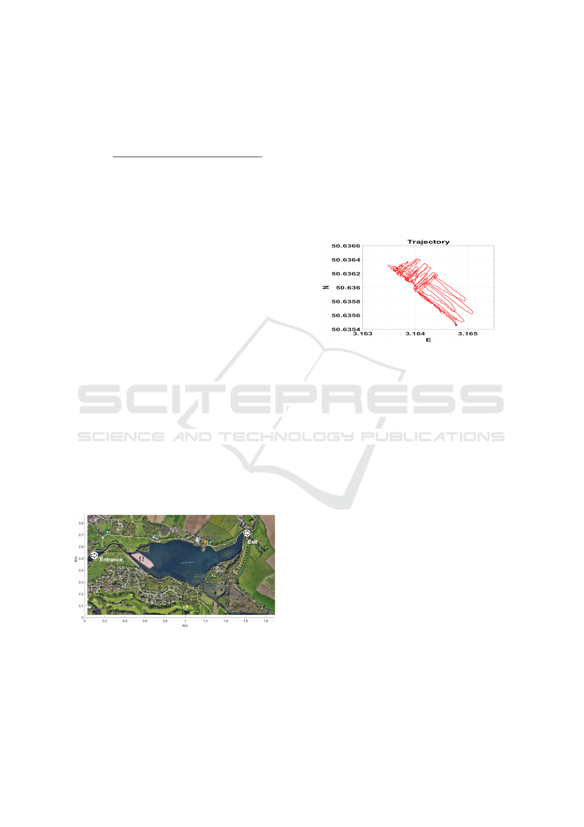
in a particular region of the Heron Lake in Villeneuve

d’Ascq, France (see region Ω on Fig. 3). In this ar-

tiﬁcial lake the water arrives from east and when the

level is too high water is pumped out to a nearby river

in the far western point. A natural remediation of the

water occurs in lake so a gradient of the parameters

can be expected between points on the entrance with

a high biodegradable inputs Ivanovsky et al. (2018).

Figure 3: Region Ω on the Heron lake, Villeneuve d’Ascq,

where the measurements need to be acquire.

Remark 11 (General Objective). In this context - as

was explain on Anderson et al. (2022) - the general

objective is to construct a limnological map of the re-

gion Ω, i.e., a map F : Ω → R

such that F assigns to

every point on Ω its approximation value of pH, tur-

bidity, conductivity, temperature and dissolved oxy-

gen (see Fig. 5 for dissolved oxygen).

The construction of map F on the region of inter-

est was discussed on Anderson et al. (2022), where an

approximation of F was proposed by geo-statistical

interpolation methods based on real measurements

provided by a hand-operated USV. The interpolation

method was necessary at this point in order to com-

plete uncovered points (unmeasured positions) due to

the irregularity of the hand-operated trajectory (see

Fig. 4).

Figure 4: Trajectory of the hand-operated vessel in region

Ω with decimal GPS coordinates.

To improve the data collection of the aforemen-

tioned physicochemical parameters, in what follows

the proposed control strategy is performed for a regu-

lar exploration of region Ω.

6.2 Motion Planning

The area of interest Ω was computed by the largest

convex set containing the entire data collection of Fig.

5. The design of the path to explore the complete re-

gion is based on a regular map meshing of Ω. The

map meshing consists in a collection of disjointed sets

{Ω

}

j=1

such that ∪Ω

contains the region Ω. The

size of every Ω

must be considered according the

size of the vessel, the accurate of the map F, the time

for the exploration mission, etc. On the other hand,

the shape of Ω

must be chosen according the best

performance of the controller. Figure 6 shows a mo-

tion planning for squares Ω

with a size of 100m

. A

discussion about the shapes and sizes of the meshing

is discussed on Anderson et al. (2022)

The controlled vessel reaches every set Ω

and

performes a direct in situ measurement of each pa-

rameters. The limnological map F is constructed by

this process.

Remark 12. The path

Ω = {Ω

,· · · ,Ω

} is an or-

dered sequence that determines in which order the

target sets Ω

are reached. According to the mesh-

ing considered in this work, there are several possible

Nonlinear Set-based Model Predictive Control for Exploration: Application to Environmental Missions

235

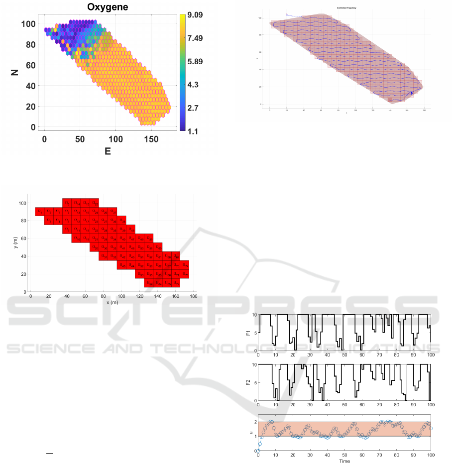
Figure 5: Limnological map F on Ω for the Dissolved Oxy-

gen (Anderson et al., 2022).

Figure 6: A motion planning to explore Ω.

regular paths for exploration; a proper motion path

would depend on the position of the initial state, wind,

water ﬂow, etc.

6.3 Exploring Results

Fig. 7 shows the application of the proposed MPC

with a prediction horizon N = 15, a discretization

of the dynamical model (9) with discrete-time with

T = 1seg and initial state x(0) = (x, y,ψ,u,v, r) =

(20,105, −

,0, 0, 0). To explore region Ω a regular

meshing of squares with a size of 25m

is used. Ev-

ery target set Ω

share an edge with the next target set

Ω

, so once the system enter into Ω, only the second

mode of the MPC (8) is used (the ﬁrst mode is only

used at the beginning to reach Ω

). Fig. 7 shows the

controlled trajectory that reach every target set Ω

least one time.

In order to construct the map F by direct in situ

measurements of each parameters inside every target

set Ω

, the velocity u of the vessel must belongs to

certain range to allows the sensor to take every mea-

surement inside Ω

for all j = 1,. ..,K. This can be

approach by considering target sets of three dimen-

Figure 7: Controlled trajectory for exploring region Ω.

sions, i.e. if z = (x, y,ψ,u,v, r)

Ω

= {z ∈ R

: l

≤ x ≤ u

, l

≤ y ≤ u

,. . .

≤ u ≤ u

, ∞ ≤ ψ,v,r ≤ ∞}.

Note that there is no consideration to minimize states

ψ,v and r, which means that they are free. For the

simulations on Fig. 8 we consider that 1 ≤ u ≤ 2

for all Ω

, j = 1 .. . ,K, i.e., proj

Ω

= [1,2] for all

j. The ﬁgure shows the velocity state and inputs

for the time interval [0,100]. On the other hand, for

the simulations on Fig. 9 the target set for the ve-

locity is 0.5 ≤ u ≤ 1.5 for all Ω

, j = 1 . .., K, i.e.,

proj

Ω

= [0.5,1.5] for all j.

Figure 8: Inputs and velocity state for the target set

proj

Ω

= [1,2].

Remark 13. Simulation results suggest that the ex-

ploration of the region of interest Ω can be done with

a very simple motion planing and with an optimal tra-

jectory that reaches every point on the surface where

a measurement needs to be performed. Even more,

the velocity of the vessel can be selected for every tar-

get Ω

with j = 1. ..,K according the requirements

of the experiment. However, more simulation experi-

ments need to be done before the real implementation,

but they are out of the scope of this work.

ICINCO 2022 - 19th International Conference on Informatics in Control, Automation and Robotics

236

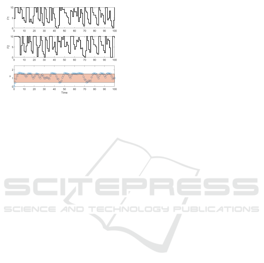
Figure 9: Inputs and velocity state u for the target set

proj

Ω

= [0.5,1.5].

7 CONCLUSION

Environmental missions were performed on Heron

Lake in Villeneuve d’Ascq, France. The main goal of

the experiment is to construct a temporal water qual-

ity proﬁle of a region of the lake, where there is a sus-

picion of a source of pollution, so more experiments

are expected in the same region. To outperformed the

data collection results, in this paper a nonlinear MPC

for USV for exploration was presented. The strategy

shows that a simple schedule of mission planning can

be obtained, and the simulations proves that large wa-

ter surfaces can be tracked in an optimal and ﬂexible

way. This results are expected to outperformed the

real exploration of large areas targeting data collec-

tion for water quality analysis.

ACKNOWLEDGEMENTS

Authors want to thanks the company https:

//www.bathydronesolutions.com/Bathy drone Solu-

tions (BDS) for its participation in the experiments,

and the Department of Economic Transformation,

Industry, Knowledge and Universities of the An-

dalusian Government (PAIDI 2020) [Ampliaci

Aquacollect, ref. P18-HO-4713].

REFERENCES

Anderson, A., Gonz

alez, A. H., Ferramosca, A., and Kof-

man, E. (2018). Finite-time convergence results in ro-

bust model predictive control. Optimal Control Appli-

cations and Methods, 39(5):1627–1637.

Anderson, A., Martin, J., Mougin, J., Bouraqadi, N., Du-

viella, E., Etienne, L., Fabresse, L., Langueh, K.,

Lozenguez, G., Alary, C., Billon, G., Superville, P.,

and Maestre, J. (2022). Water Quality Map Extraction

from Field Measurements Targetting Robotic Simula-

tions. working paper or preprint.

Bertrand, S., Marzat, J., Piet-Lahanier, H., Kahn, A., and

Rochefort, Y. (2014). MPC strategies for coopera-

tive guidance of autonomous vehicles. Aerospace Lab,

(8):1–18.

Blanchini, F. and Miani, S. (2015). Set-Theoretic Methods

in Control. Systems & Control: Foundations & Ap-

plications. Springer International Publishing.

Goerzen, C., Kong, Z., and Mettler, B. (2010). A survey of

motion planning algorithms from the perspective of

autonomous uav guidance. Journal of Intelligent and

Robotic Systems, 57(1):65–100.

Hervagault, Y. (2019). Design and Implementation of an Ef-

fective Communication and Coordination System for

Unmanned Surface Vehicles (USV). PhD thesis, Uni-

versit

e Grenoble Alpes.

Ivanovsky, A., Belles, A., Criquet, J., Dumoulin, D., Noble,

P., Alary, C., and Billon, G. (2018). Assessment of

the treatment efﬁciency of an urban stormwater pond

and its impact on the natural downstream watercourse.

Journal of Environmental Management, 226:120–130.

Limon, D., Alamo, T., and Camacho, E. F. (2005). Enlarg-

ing the domain of attraction of mpc controllers. Auto-

matica, 41(4):629–635.

Lindqvist, B., Mansouri, S. S., and Nikolakopoulos, G.

(2020). Non-linear mpc based navigation for micro

aerial vehicles in constrained environments. In 2020

European Control Conference (ECC), pages 837–842.

IEEE.

Matschek, J., B

athge, T., Faulwasser, T., and Findeisen,

R. (2019). Nonlinear predictive control for trajectory

tracking and path following: An introduction and per-

spective. In Handbook of Model Predictive Control,

pages 169–198. Springer.

Nascimento, T. P. and Saska, M. (2019). Position and atti-

tude control of multi-rotor aerial vehicles: A survey.

Annual Reviews in Control, 48:129–146.

Nigam, N. (2014). The multiple unmanned air vehicle per-

sistent surveillance problem: A review. Machines,

2(1):13–72.

Prodan, I., Olaru, S., Bencatel, R., de Sousa, J. B.,

Stoica, C., and Niculescu, S.-I. (2013). Receding

horizon ﬂight control for trajectory tracking of au-

tonomous aerial vehicles. Control Engineering Prac-

tice, 21(10):1334–1349.

Sarunic, P. and Evans, R. (2014). Hierarchical model

predictive control of uavs performing multitarget-

multisensor tracking. IEEE Transactions on

Aerospace and Electronic Systems, 50(3):2253–2268.

Nonlinear Set-based Model Predictive Control for Exploration: Application to Environmental Missions

237