
Sampling Strategies for Static Powergrid Models
Stephan Balduin
a
, Eric MSP Veith
b
and Sebastian Lehnhoff
c
OFFIS - Institute for Information Technology, Escherweg 2, Oldenburg, Germany
Keywords:
Machine Learning, Power Grid, Power Flow, Surrogate Models, Sampling, Correlation.
Abstract:
Machine learning and computational intelligence technologies gain more and more popularity as possible
solution for issues related to the power grid. One of these issues, the power flow calculation, is an iterative
method to compute the voltage magnitudes of the power grid’s buses from power values. Machine learning
and, especially, artificial neural networks were successfully used as surrogates for the power flow calculation.
Artificial neural networks highly rely on the quality and size of the training data, but this aspect of the process
is apparently often neglected in the works we found. However, since the availability of high quality historical
data for power grids is limited, we propose the Correlation Sampling algorithm. We show that this approach
is able to cover a larger area of the sampling space compared to different random sampling algorithms from
the literature and a copula-based approach, while at the same time inter-dependencies of the inputs are taken
into account, which, from the other algorithms, only the copula-based approach does.
1 INTRODUCTION
The knowledge about the current state of the power
grid is usually limited to information about the power
generation or consumption of the grids’ participants,
either through prognosis or by estimations via default
load profiles. However, a stable grid operation re-
quires a certain frequency level (50 Hz in Europe) and
certain voltage levels. Since only the power values are
known, voltage information needs to be calculated,
which is done with Power Flow (PF) analysis (Pow-
ell, 2004). The PF analysis is performed many times
during the operation of power grid,s and the results
can be used, e. g., for market analysis or short-term
operational planning.
Since the PF analysis often requires performing
matrix inversion, a task with a high computational
burden, there are many approaches to reduce this
computation time. Besides improvements for the tra-
ditional methods, the advancement and application
of Machine Learning (ML) models for energy sys-
tems have also increased in the past two decades. Al-
though the number of papers that solely focus on PF
is rather small (Hasan et al., 2020), there are many
works about the closely related optimal PF and proba-
bilistic PF, which are specific use cases for PF. Artifi-
a
https://orcid.org/0000-0002-2018-1078
b
https://orcid.org/0000-0003-2487-7475
c
https://orcid.org/0000-0003-2340-6807
cial neural networks are used with great performance
for various PF-related problems. However, artificial
neural networks require a large amount of data, espe-
cially when several hidden layers are used.
In our previous works in (Balduin et al., 2019;
Balduin et al., 2020), we built a deep neural network
to avoid the costly PF for a low voltage power grid
model. One issue we identified concerns the availabil-
ity of power system data that can be used for training.
Therefore, we decided to take a deeper look at the
available data sets and sampling algorithms in the lit-
erature.
The contribution of this paper is two-fold. First,
we are pointing out the challenges and pitfalls of
retrieving training data for a power grid simulation
model and how different approaches in the literature
handled this. Second, we present the correlation-
based approach that we built to overcome some of
those issues.
The rest of this paper is structured as follows. In
section 2 we present the results of our investigation
and discuss relevant literature. The simulation model
is described in section 3, section 4 provides some of
the basics of sampling strategies, and in section 5 we
discuss the challenges of applying sampling strategies
to power grid models. In section 6, we present our
Correlation Sampling approach, which we compare
and discuss in section 7. We conclude our paper in
section 8.
Balduin, S., Veith, E. and Lehnhoff, S.
Sampling Strategies for Static Powergrid Models.
DOI: 10.5220/0011306400003274
In Proceedings of the 12th International Conference on Simulation and Modeling Methodologies, Technologies and Applications (SIMULTECH 2022), pages 319-326
ISBN: 978-989-758-578-4; ISSN: 2184-2841
Copyright
c
2022 by SCITEPRESS – Science and Technology Publications, Lda. All rights reserved
319

2 RELATED WORK
The Open Power System Data platform (Wiese et al.,
2019) provides a hub for different data sets that can be
used for electricity system modeling. In their work,
the authors criticize that the quality and accessibil-
ity of publicly available data sets is often inadequate,
require different files to download, have poor docu-
mentation, or are erroneous. This is different for the
data sets provided or linked on the Open Power Sys-
tem Data platform; however most concern power gen-
eration. The available load data sets are highly ag-
gregated hourly or monthly time series or small-scale
household data sets. Another good overview of data
sets, especially for distribution grids, can be found in
the wiki of the openmod initiative
1
. The Simbench
project (Spalthoff et al., 2019) provides a large data
set, ranging over all German voltage-levels, contain-
ing time series for loads and generation. Finally, there
are the IEEE test cases, which mainly focus on North-
American-style systems.
Besides using publicly available datasets some
works propose methodologies to create synthetic
datasets. (H
¨
ulk et al., 2017) used annual consumption
data to generate a synthetic data set of the German
energy system. This was extended by (Amme et al.,
2018) with a focus on the medium-voltage grid level.
Likewise, in the research project SmartNord (Blank
et al., 2015), a methodology was proposed to generate
synthetic household loads that, once aggregated, fol-
low the German default load profile H0, which grid
operators use.
When neither of the above mentioned data sets
fit or the data set is not large enough, sampling may
be the solution. While this originates in the field of
probabilistic PF, where inputs of the PF calculation
are modeled as random variables (Chen et al., 2008),
sampling is used in other PF-related fields as well.
(Cai et al., 2013) use polynomial normal transforma-
tion together with Latin Hypercube sampling to build
probability distribution models for probabilistic PF.
Their models were able to handle correlated inputs
and achieved better results on the IEEE 14-bus and
118-bus systems compared to a Simple Random Sam-
pling (SRS) approach. Also in the field of probabilis-
tic PF, (Huang et al., 2020) sampled with Latin Hy-
percube sampling as well but used D-vine copulas to
model the inter-dependencies of wind speed between
four wind farms. They evaluated the approach on a
modified IEEE 33-bus system against SRS.
(Lei et al., 2020) used a Monte-Carlo simulation
1
https://wiki.openmod-initiative.org/wiki/
Distribution network datasets, retrieved on 07 Apr.
2022
approach combined with an interior point algorithm
to obtain feasible samples for optimal PF. They also
did a sample pre-classification to group samples that
share the same active constraints. The test cases were
carried out on the IEEE 39, 57, and 118-bus systems
as well as on a Polish 2383-bus system. Some works,
especially in the field of optimal PF simply use the
base load values provided with most power grid mod-
els, e. g., the works in (Guha et al., 2019) and (Pan
et al., 2019) use 10% and (Zamzam and Baker, 2020)
even 70% deviation of the base load, although they, at
least, did not sample from a uniform distribution.
In (Thayer and Overbye, 2020), the authors sam-
pled a variation of the overall consumption and indi-
vidual scaling factors for each load on the IEEE 14-
bus system. Afterwards, loads are summed up and lin-
early scaled to match the overall consumption. Their
use case was voltage control based on deep reinforce-
ment learning. Quite similar is the work of (Diao
et al., 2019). However, the authors used the base load
of the IEEE 14-bus system and created a load fluctua-
tion between 80 % and 120 % of the base load values.
From this literature research we conclude that
there are a couple of data sets available as well as
several ways to generate synthetic data sets. Unfor-
tunately, those data sets comprise not more than one
year of data. Furthermore, we found different ap-
proaches to directly sample the power grid model,
predominantly one of the IEEE test cases, from dif-
ferent research fields. Some of the works we have
discussed consider actual time series of, e. g., wind
farms for generation, others simply used the base load
for sampling. The resulting sampling data has a high
chance to have completely different distributions than
realistic (or synthetic) data, which can affect the qual-
ity of a prediction model. To this end, we propose
a methodology that takes into account realistic time
series and their inter-dependencies while at the same
time preserve the flexibility of the sampling proce-
dure.
3 SIMULATION MODEL
We used the Python library pandapower (Thurner
et al., 2018), which allows to model arbitrary power
grid topologies and is able to perform a power flow
calculation for that topology given a set of input data
for all relevant nodes. To setup the simulation, a
grid model is instantiated and a data set is loaded.
We used a power grid from the Simbench project
(1-LV-rural3--0-sw), because they have data sets
included that are explicitly tailored for the grid topol-
ogy. The simulation loop consists of assigning input
SIMULTECH 2022 - 12th International Conference on Simulation and Modeling Methodologies, Technologies and Applications
320

values (active and reactive power) from the data set to
the corresponding nodes of the power grid, perform-
ing the power flow calculation, and then saving the
results from the buses: voltage magnitude per unit
(although not used for this paper), active, and reac-
tive power. This process is repeated until all entries
of the data set are simulated.
4 SAMPLING STRATEGIES
Since the model described above is a computer-based
simulation model, the design of experiments literature
would recommend space-filling designs (Dean and
Voss, 1999). Such designs aim to spread the sample
points for each input evenly in the sample space. This
can be achieved with Monte Carlo Sampling (some-
times also called Simple Random Sampling (SRS)),
i. e., using the uniform distribution independently for
each input. Given that enough samples were drawn,
this approach creates nearly orthogonal sampling de-
signs i. e., the inputs are uncorrelated.
In general, orthogonality and uniformly dis-
tributed inputs are desired properties of a sampling
design since they can improve the validity of the pre-
diction model created from that design. However,
there are cases where some of the inputs in the origi-
nal system-under-investigation are correlated and the
power grid is a prime example for this. To build a
model that captures this behavior, the sample distri-
butions for those inputs need to be correlated as well.
One solution is to use Copulas, which were first pro-
posed by (Sklar, 1959). Copulas can handle marginal
distributions of random variables and dependencies
separately. That is why an increasing number of pub-
lications that have to deal with dependencies in power
system modeling use Copulas.
5 CHALLENGES OF POWER
GRID SAMPLING
The power grid is a complex system, i. e., the more
basic approaches from the design of experiments lit-
erature for sampling and analysis cannot be applied
to the power grid model without modifications. The
complex inter-dependencies between the parts of the
power grid make it hard to guarantee properties like
orthogonality or uniformly distributed marginal dis-
tributions of the inputs without risking a decrease of
the quality of the prediction model. Not considering
specific correlations could even lead to ill-conditioned
states of the power grid, where the PF calculation
fails.
(Gerster et al., 2021) investigated sampling strate-
gies for the determination of flexibility potentials at
vertical system interconnections. One of their ma-
jor conclusions concerns the application of uniform
sampling for each of the inputs. With an increasing
number of inputs, the samples suffer more and more
from the convolution problem (Bremer and Lehn-
hoff, 2018), i. e., at the vertical system interconnec-
tion point the actually covered space on the P-Q plane
gets smaller the more inputs are involved.
Another challenge concerns the definition of the
sample space of the inputs. While for most inputs,
zero can be considered as minimum value, the maxi-
mum is not clearly defined. The base value attached
to the publicly available power grid models and test
cases may serve as reference value. However, it is not
a maximum value since calculating the PF using base
loads usually results in a healthy or, depending on the
test case, slightly violated system state. It is also not
an average value, which can be seen at the distribu-
tions of realistic load or generation profiles.
The advantage of using the base load as reference
and creating samples around those values with a spe-
cific deviation is that just the grid model itself without
any time series data is required. This makes it conve-
nient if only the general capabilities of an ML model
should be explored. However, unless the ML model
is at least evaluated on realistic data, the model may
only be a showcase for a certain ML algorithm on an
environment that happens to be a power grid model.
It does not necessarily imply that this model still per-
forms well if realistic data is used.
Figure 1: Active power time series of the load connected to
bus 42 (randomly selected) over one year of simulated time.
Taken from the Simbench grid 1-LV-rural3--0-sw.
Figure 1 illustrates the active power of a randomly
selected household of the power grid described in sec-
tion 3. The maximum peak power is 3 kW, which is
the nominal power of the corresponding load in the
grid model. In Figure 2 we plotted the histogram of
Sampling Strategies for Static Powergrid Models
321
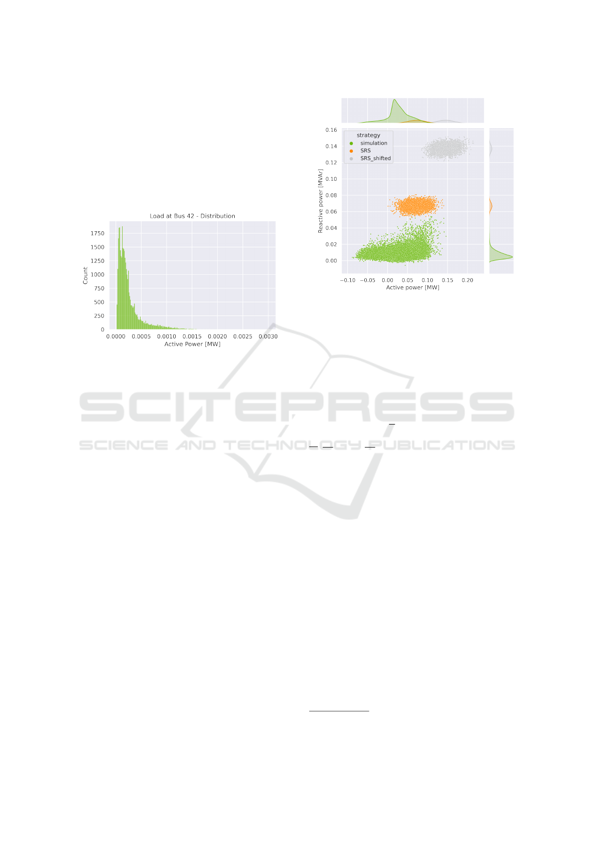
this time series. Now it becomes obvious that most
of the data is between 0.0 and 0.5 kW. Actually, the
mean value is ≈ 0.2657, the standard deviation ≈
0.2781, and the median is ≈ 0.1835. Sampling around
the base load of 3 kW would result in samples that,
although valid, do not represent the original data and,
consequently, which do not contain the necessary in-
formation for a ML model that should make predic-
tions based on realistic input data.
Figure 2: Histogram of the same active power time series as
in Figure 1.
Next, we simulated the power grid for one year
of simulated time. We followed (Gerster et al., 2021)
and plotted active against reactive power at the slack
bus to get an estimate of the distribution of all of the
simulation data and to be able to detect possible con-
volution problems. This can be seen in Figure 3.
Now, we wanted to evaluate how well different
sampling algorithms from the literature perform for
this data set. We started with two variants of the SRS
method; the first samples between 0 and the base load
(Equation 1) and the second samples around the base
load with a certain δ (Equation 2).
p
∗
∼ Uniform[0,p
b
] (1)
p
∗
∼ Uniform[(1 − δ) · p
b
,(1 + δ) · p
b
] (2)
Here, p
b
is the vector of base loads in the grid, δ is
the deviation from the base load, and p
∗
is the vector
of sampled power values. We used this formulas to
generate 5000 samples for active and reactive power
consumption as well as active power generation (the
generators of the grid in-use had reactive power set to
zero) with a δ of 0.5 in the second case. Afterwards,
we calculated the PF for all samples to obtain the
active and reactive power for the slack bus, just like
above. The results can be seen in Figure 3. While all
of the samples were feasible (i. e., the PF converged),
we see that those distributions did not match at all.
Figure 3: Plot of the P-Q plane at the slack bus. The lower
dot cloud represents the results from original data sets. The
middle dot cloud represents the results from the first SRS
variant (sampling between zero and the base load) and the
upper dot cloud the results from the second SRS variant
(sampling around the base load).
A more advanced sampling strategy was used by
(Thayer and Overbye, 2020). First, the authors used
Equation 1 to sample active power on the interval [0.0,
1.0). Next, they varied the total active power loading
P
0
uniformly between 60 % and 140% of the total ac-
tive power loading P calculated from the base load.
Each of the loads is scaled linearly with the factor
P
0
/P
∗
where P
∗
is the total active power calculated
from the samples p
∗
. For reactive power Q, a power
factor p f for each load is drawn uniformly on the in-
terval [0.8, 1.0) and Q is calculated with
Q = P · tan(arccos(p f )) · L,L ∈ {−1, 1}. (3)
The factor L is a random variable with a chance of
10% to be -1 and, therefore, to flip the sign of Q. Like
before, we created 5000 samples and calculated the
PF results. The P-Q plot is shown in Figure 4. While
a much larger part of the sampling space is covered,
the areas of the original data and the sample data were
completely different.
Finally, we created a Gaussian copula to perform
the same task. We used the python package copulas
2
,
which provides appropriate functions. The result is
shown in Figure 4. The copula samples cover most of
the space that is covered by the original data as well.
We performed this experiment with different grid
models and different time series and got similar re-
sults. Our conclusion is that SRS-based approaches
2
https://sdv.dev/, retrieved on 14 Apr. 2022
SIMULTECH 2022 - 12th International Conference on Simulation and Modeling Methodologies, Technologies and Applications
322

Figure 4: The results of the advanced and the copula-based
sampling were added to the plot. The darker dot cloud on
top of the dot cloud of original data shows that copulas were
able to reproduce the behavior of the original data.
are fine when no realistic data sets are available or the
model prediction model will not not be used with re-
alistic data sets. In any other case, copulas allow to
create samples that represent the realistic data set.
However, there is one additional concern related
to our specific use case. The copula samples might
match the realistic data too well. One of the de-
sired properties for sampling designs is that the sam-
ple points are evenly spread over the whole sample
space. Although we don’t know the real boundaries of
the sampling space, the SRS-based approaches cover
valid areas of the sampling space that are not covered
by the copula samples. We address this shortcoming
with our sampling algorithm.
6 CORRELATION SAMPLING
The correlation sampling approach consists of two
parts. In the first part, the correlations between the
inputs are calculated and, int the second part, those
correlations are used to create a sampling design.
6.1 Correlations
Naturally, the different entities that are connected to
the power grid have inter-dependencies. Households
follow similar patterns although there are different
types of profiles. Photovoltaic modules are heavily
dependent on the time of the day and weather condi-
tions like cloudiness and solar radiation, which results
in high correlations at spatially close positioned mod-
ules. Correlation can also be found between commer-
cial facilities like different super markets or between
several heating devices, which are dependent on tem-
perature conditions.
Utilizing those inter-dependencies is also done in
(Huang et al., 2020) to sample wind power plants for
probabilistic PF and in (Blank, 2015) to assess the re-
liability of coalitions for the provision of ancillary ser-
vices. Those inter-dependencies can also be found in
the time series data sets for power grids, at least when
the data set aims to be realistic. Therefore, we de-
cided to use correlations, or, more specific partial cor-
relations, to generate samples. The widely used cor-
relation coefficient by Pearson (Benesty et al., 2009)
is defined as
r
XY
=
cov(X,Y )
σ
X
σ
Y
(4)
with X,Y being random variables, σ
X
,σ
Y
the stan-
dard deviation of X and Y and cov is the covariance.
When more than two random variables are involved,
other variables Z = (Z
1
,...,Z
n
) may have correlation
to X and Y as well. Especially, Z
i
might be related to
both X and Y . To get the unbiased correlation between
X and Y , the partial correlation can be calculated with
r
XY |Z
i
=
r
XY
− r
XZ
i
· r
Y Z
i
q
1 − r
2
XZ
i
·
q
1 − r
2
Y Z
i
(5)
This can be described as two linear regression
problems, the first between Z
i
and X and the second
between Z
i
and Y (Whittaker, 2009). Since the resid-
uals of those linear regressions are uncorrelated to Z
i
,
the sample correlation can be calculated to obtain the
partial correlation between X and Y .
We will illustrate this using the data set from the
Simbench grid that was already used in the previous
chapter. The Partial Correlation Matrix (PCM) C be-
tween all of the inputs for the power grid over the en-
tire data set, displayed as heat map, can be seen in
Figure 5.
Although this PCM is sufficient for our sampling
algorithm, we still used the whole data set to calcu-
late the correlations. To overcome this, we selected a
subset of the data set containing 2500 samples
3
and
calculated the PCM as C
0
again. This heat map can be
seen in Figure 6.
If you take a close look at both heat maps, you
probably recognize similar ”patterns”. In fact, those
PCMs are quite similar with a correlation factor of
r
CC
0
= 0.98, with duplicates (the lower left triangle
of the matrix) included. The accumulated point-wise
3
This number is arbitrarily chosen and may only fit the
current use case.
Sampling Strategies for Static Powergrid Models
323
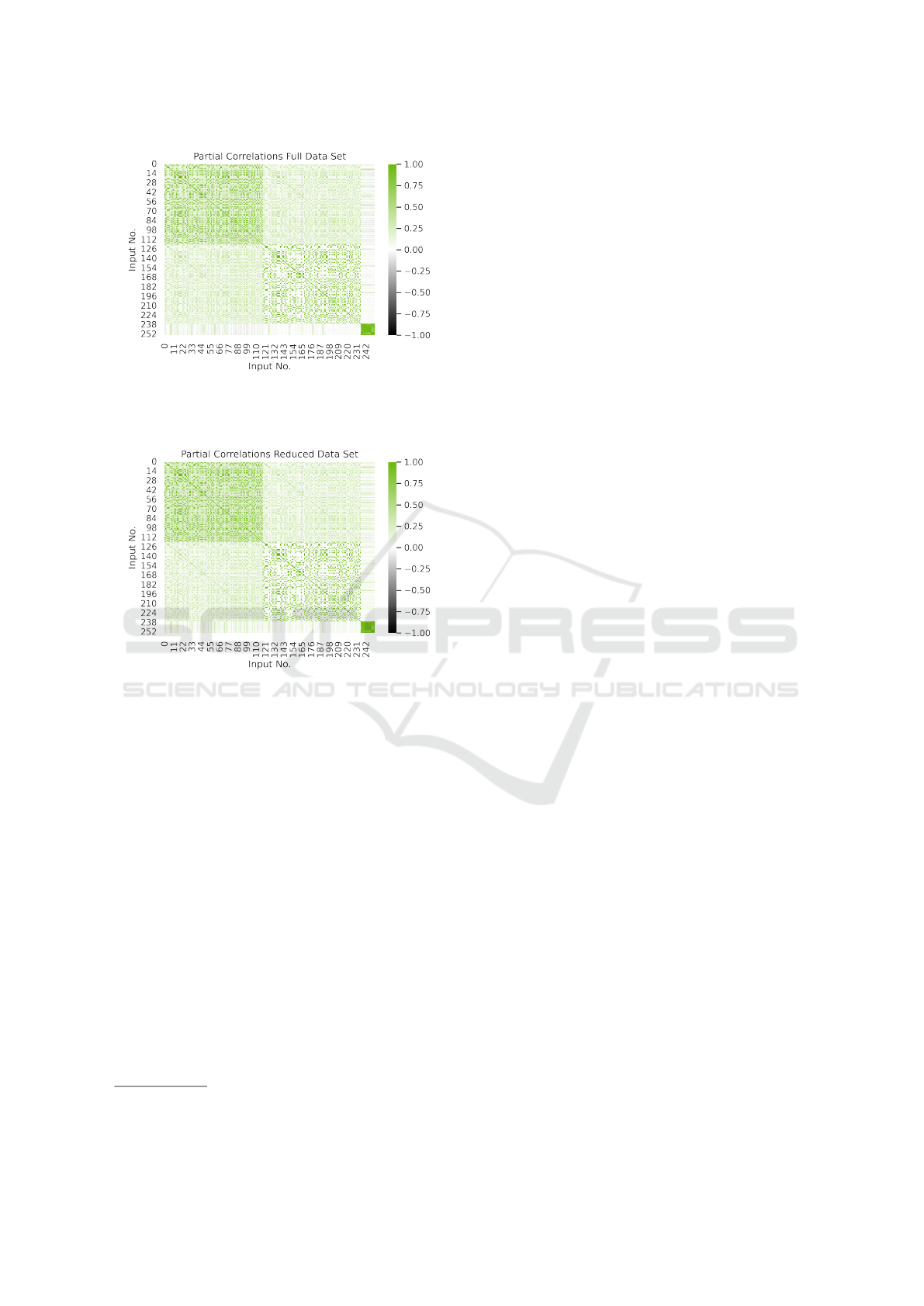
Figure 5: Heat map to illustrate the partial correlations
between the inputs of data set provided by the Simbench
power grid.
Figure 6: In contrast to Figure 5, the correlations are calcu-
lated from a small subset of the data.
difference C - C
0
sums up to -391.6 with a mean of -
0.006, which indicates that the reduced PCM slightly
over-estimates positive correlations. With a standard
deviation of 0.055, we concluded that the reduced
PCM is similar enough
4
.
6.2 Sampling
The next step concerned how to integrate the PCM C
0
into the sampling procedure. Most of the partial cor-
relations are lower than 0.5 but there is another clus-
ter between ≈ 0.85 and 1.0. To not suppress the ran-
domness of the sampling, we defined a threshold t of
0.85 and ignored all correlations that were lower with
their absolute value. Each sample s is initially gen-
erated with the Dirichlet distribution, which was used
by (Gerster et al., 2021) with good results. For each
sample s
i
in s, all subsequent entries s
j
with i < j, are
adapted depending on their partial correlation C
0
i j
:
4
This may depend on the data sets in-use. For our use
case, the similarity was sufficient
s
j
=
s
j
, |C
i j
| < t
s
i
+ s
j
· (1 −C
i j
), C
i j
> 0
1 − s
i
+ s
j
· (1 +C
i j
), C
i j
< 0
(6)
The general idea is to pull the value of sample s
j
towards the value of sample s
i
if they’re highly corre-
lated. In Equation 6, cases two and three account for
positive and negative correlation respectively.
We also applied some additional optimizations to
better suit the current use case. First of all, we multi-
plied s
j
with a normal distributed noise factor of 10%
in cases where the correlation exceeds the threshold
to relax the linear dependency towards s
i
. Second, to
overcome some of the issues we’ve seen at the other
sampling approaches, we calculated the sum of all
values of this sample s and compared it to an interval
[s
min
, s
max
]. When s is not in [s
min
, s
max
], s is discarded
and sampled again.
The values s
min
and s
max
are derived from the data
set again, by normalizing each time series individu-
ally, then building the sum for each time step, and,
finally, assigning the minimum value to s
min
and the
maximum value to s
max
. However, since we used a re-
duced data set and, therefore, the interval [s
min
, s
max
]
may be to small, we extended it by 20 % in each di-
rection.
7 EVALUATION
7.1 Results
We used the described methodology to create samples
like we did for the other sampling strategies. The P-
Q plot at the slack bus is shown in Figure 7. It can
be seen that the correlation samples not only cover
the space of the real data but are also located in the
regions largely around the real data. This even in-
cludes most of the space covered by the other sam-
pling strategies.
The correlation between the copula-sampled PCM
and the original full-data PCM is ≈ 0.98, which
matches the correlation of the PCM of the reduced
data set. For the correlation-sampled PCM, the is ≈
0.864, which is less than the reduced data set but still
very high. However, this difference may be one of the
reasons why a larger area is covered.
We repeated this comparison with another power
grid model, the CIGRE low voltage benchmark grid,
in combination with synthetic time series data from
Smart Nord, since we used this model in our previous
works already. The results are shown in Figure 8 and
this resembles all the issues and conclusions we iden-
SIMULTECH 2022 - 12th International Conference on Simulation and Modeling Methodologies, Technologies and Applications
324
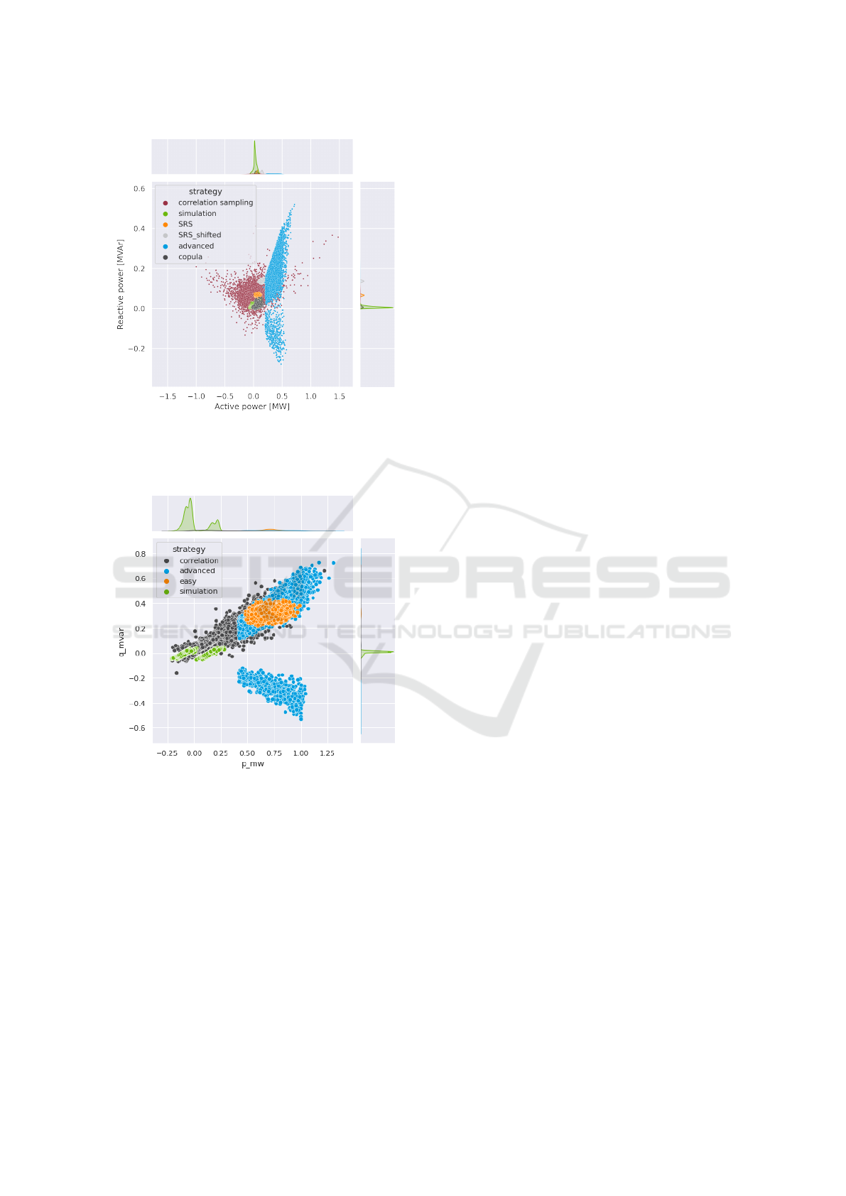
Figure 7: The results of the correlation samples are added
to the P-Q plot. A large area around the original data is
covered, which includes even the areas of most of the other
sampling algorithms.
Figure 8: The P-Q plot with different sampling algorithms
for the CIGRE low voltage grid.
tified for the Simbench grid, although the data sets are
completely independent of each other.
7.2 Discussion
The correlation sampling approach is, in its current
state, a subject of experimentation. There are sev-
eral parameters, like the correlation threshold or the
number of samples that are used to calculate the par-
tial correlations, which were determined experimen-
tally and not for a special mathematical reason. There
might be parameters that even lead to better results.
Furthermore, only linear correlations are considered
but in the data sets might be nonlinear correlations
as well, which could be utilized to get more accurate
samples.
On the other side, correlation sampling solved the
issue we had with other sampling strategies. It covers
the areas of the original data in the output space and,
at the same, the regions beyond as well. In theory, this
improves a prediction model’s capabilities to general-
ize when some parameters in the grid configuration
have changed. However, this is beyond the scope of
this paper.
8 CONCLUSION
In this paper, we presented a small literature research
about available data sets for power system modeling,
where to find them, and discussed some of the issues
some of those data sets have. We also reviewed al-
gorithms from the literature that were used to sam-
ple data sets for power grid simulation models and
pointed out advantages and disadvantages.
The main issue of those strategies that neglect
inter-dependencies is that created samples cover en-
tirely different areas of the output space considering
the P-Q plane at the grid interconnection point. A pre-
diction model trained with those samples will most
probably fail when more realistic type of data will
be used as prediction input. On the other side, cop-
ulas resemble the original data very well and we rec-
ommend them as first choice whenever a prediction
model should be used in a context with realistic data.
Furthermore, we presented our Correlation Sam-
pling approach that aims to not only cover the ”re-
alistic” areas of the output space by taking inter-
dependencies between the inputs into account. But
also to cover the regions beyond to improve the gen-
eralization capabilities of the model.
Although those first results looks promising, we
see a lot of potential for improvements of the algo-
rithm. Additionally, the data set created with correla-
tion sampling still needs to be used to build a surro-
gate model, which is the primary purpose we devel-
oped that algorithm. We will present the results from
those experiments in future work.
ACKNOWLEDGEMENTS
This work was funded by the German Federal Min-
istry of Education and Research through the project
PYRATE (01IS19021A).
Sampling Strategies for Static Powergrid Models
325

REFERENCES
Amme, J., Pleßmann, G., B
¨
uhler, J., H
¨
ulk, L., K
¨
otter, E.,
and Schwaegerl, P. (2018). The ego grid model: An
open-source and open-data based synthetic medium-
voltage grid model for distribution power supply sys-
tems. In Journal of Physics: Conference Series, vol-
ume 977, page 012007. IOP Publishing.
Balduin, S., Tr
¨
oschel, M., and Lehnhoff, S. (2019). Towards
domain-specific surrogate models for smart grid co-
simulation. Energy Informatics, 2(1):1–19.
Balduin, S., Westermann, T., and Puiutta, E. (2020). Eval-
uating different machine learning techniques as sur-
rogate for low voltage grids. Energy Informatics,
3(1):1–12.
Benesty, J., Chen, J., Huang, Y., and Cohen, I. (2009).
Pearson correlation coefficient. In Noise reduction in
speech processing, pages 37–40. Springer.
Blank, M. (2015). Reliability Assessment of Coalitions for
the Provision of Ancillary Services. PhD thesis, Uni-
versit
¨
at Oldenburg.
Blank, M., Breithaupt, T., Bremer, J., Dammasch, A.,
Garske, S., Klingenberg, T., Koch, S., L
¨
unsdorf, O.,
Niesse, A., Scherfke, S., Hofmann, L., and Sonnen-
schein, M. (2015). Smart nord final report. Technical
report, Uni Hannover.
Bremer, J. and Lehnhoff, S. (2018). Unfolding ensemble
training sets for improved support vector decoders in
energy management. In ICAART (2), pages 322–329.
Cai, D., Shi, D., and Chen, J. (2013). Probabilistic load flow
computation with polynomial normal transformation
and latin hypercube sampling. IET Generation, Trans-
mission & Distribution, 7(5):474–482.
Chen, P., Chen, Z., and Bak-Jensen, B. (2008). Probabilistic
load flow: A review. In 2008 Third International Con-
ference on Electric Utility Deregulation and Restruc-
turing and Power Technologies, pages 1586–1591.
IEEE.
Dean, A. and Voss, D. (1999). Design and analysis of ex-
periments. Springer.
Diao, R., Wang, Z., Shi, D., Chang, Q., Duan, J., and
Zhang, X. (2019). Autonomous voltage control for
grid operation using deep reinforcement learning. In
2019 IEEE Power & Energy Society General Meeting
(PESGM), pages 1–5. IEEE.
Gerster, J., Lehnhoff, S., Sarstedt, M., Hofmann, L., and
Veith, E. M. (2021). Comparison of random sampling
and heuristic optimization-based methods for deter-
mining the flexibility potential at vertical system in-
terconnections. In 2021 IEEE PES Innovative Smart
Grid Technologies Europe (ISGT Europe), pages 1–6.
IEEE.
Guha, N., Wang, Z., Wytock, M., and Majumdar, A. (2019).
Machine learning for ac optimal power flow. arXiv
preprint arXiv:1910.08842.
Hasan, F., Kargarian, A., and Mohammadi, A. (2020). A
survey on applications of machine learning for opti-
mal power flow. In 2020 IEEE Texas Power and En-
ergy Conference (TPEC), pages 1–6.
Huang, Y., Chen, S., Chen, Z., Hu, W., and Huang, Q.
(2020). Improved probabilistic load flow method
based on d-vine copulas and latin hypercube sampling
in distribution network with multiple wind genera-
tors. IET Generation, Transmission & Distribution,
14(5):893–899.
H
¨
ulk, L., Wienholt, L., Cußmann, I., M
¨
uller, U. P., Matke,
C., and K
¨
otter, E. (2017). Allocation of annual elec-
tricity consumption and power generation capacities
across multiple voltage levels in a high spatial reso-
lution. International Journal of Sustainable Energy
Planning and Management, 13:79–92.
Lei, X., Yang, Z., Yu, J., Zhao, J., Gao, Q., and Yu, H.
(2020). Data-driven optimal power flow: A physics-
informed machine learning approach. IEEE Transac-
tions on Power Systems, 36(1):346–354.
Pan, X., Zhao, T., and Chen, M. (2019). Deepopf: Deep
neural network for dc optimal power flow. In 2019
IEEE International Conference on Communications,
Control, and Computing Technologies for Smart Grids
(SmartGridComm), pages 1–6. IEEE.
Powell, L. (2004). Power system load flow analysis. Mc-
Graw Hill professional.
Sklar, A. (1959). Fonctions d
´
e repartition
`
a n dimension
et leurs marges. Paris: Publications de l’Institut de
statistique de l’Universit
´
e de Paris, 8:229–231.
Spalthoff, C., Sarajlic, D., Kittl, C., Drauz, S., Kneiske, T.,
Rehtanz, C., and Braun, M. (2019). Simbench: Open
source time series of power load, storage and genera-
tion for the simulation of electrical distribution grids.
In International ETG-Congress 2019; ETG Sympo-
sium, pages 1–6. VDE.
Thayer, B. L. and Overbye, T. J. (2020). Deep reinforce-
ment learning for electric transmission voltage con-
trol. In 2020 IEEE Electric Power and Energy Con-
ference (EPEC), pages 1–8. IEEE.
Thurner, L., Scheidler, A., Sch
¨
afer, F., Menke, J., Dol-
lichon, J., Meier, F., Meinecke, S., and Braun, M.
(2018). pandapower — an open-source python tool for
convenient modeling, analysis, and optimization of
electric power systems. IEEE Transactions on Power
Systems, 33(6):6510–6521.
Whittaker, J. (2009). Graphical models in applied multi-
variate statistics. Wiley Publishing.
Wiese, F., Schlecht, I., Bunke, W.-D., Gerbaulet, C., Hirth,
L., Jahn, M., Kunz, F., Lorenz, C., M
¨
uhlenpfordt, J.,
Reimann, J., and Schill, W.-P. (2019). Open power
system data – frictionless data for electricity system
modelling. Applied Energy, 236:401–409.
Zamzam, A. S. and Baker, K. (2020). Learning optimal so-
lutions for extremely fast ac optimal power flow. In
2020 IEEE International Conference on Communica-
tions, Control, and Computing Technologies for Smart
Grids (SmartGridComm), pages 1–6. IEEE.
SIMULTECH 2022 - 12th International Conference on Simulation and Modeling Methodologies, Technologies and Applications
326
