Modeling of Modified Vehicle Crashworthiness using a Double
Compound Pendulum
Gulshan Noorsumar
a
, Svitlana Rogovchenko
b
, Dmitry Vysochinskiy
c
and Kjell G. Robbersmyr
d
Department of Engineering Sciences, University of Agder, Grimstad, Norway
Keywords:
Double Pendulum, Vehicle Collisions, Torsional Spring, Lumped Parameter Model, Modified Vehicle.
Abstract:
Vehicle crash modeling has been a challenge for researchers for several decades. Occupant injury prevention
and prediction is a critical area within vehicle safety design. The modeling of material failure in structural
members during a full frontal crash has been presented in this paper. This study presents a Lumped Parameter
Model (LPM) with an elastic double compound pendulum replicating the impact kinematics. The model
defined using Lagrangian formulation; presents a novel methodology to represent material fracture caused
due to heat affected zones or welding in Ultra High Strength Steels (UHSS) in a non-linear crash event.
The material fracture leads to rotation of the vehicle; presented in the form of torsional springs in the LPM
developed in this study. The Simulink model has been validated with a finite element simulation and shows
good correlation to predict parameters crucial to design for occupant protection in a vehicle crash.
1 INTRODUCTION
Traffic accidents lead to many fatalities on the roads
worldwide. It is one of the major global problems
which demands attention. With an increasing global
population, transportation demands have increased
leading to more cars on roads and appropriate efforts
to reduce traffic related injuries should be taken. Au-
tomakers and researchers strive to achieve stringent
safety regulations improving the safety of occupants
and road users in a crash (Noorsumar et al., 2021a).
Real-time crash impacts had been the preferred mode
of safety testing for new cars for decades; the emer-
gence of mathematical models have reduced physical
testing during the development process. There is still
a need to further decrease the dependence on physical
tests for crashworthiness assessment of vehicles.
Noorsumar et al. (Noorsumar et al., 2021a) have
reviewed the mathematical models used in the indus-
try and academia to replicate vehicle impacts. Fi-
nite Element Methods (FEM) have found applications
in several areas of safety research; one of the early
contributions to the theory and applications of FEM
a
https://orcid.org/0000-0002-6718-4508
b
https://orcid.org/0000-0001-8002-4974
c
https://orcid.org/0000-0002-0453-0012
d
https://orcid.org/0000-0001-9578-7325
in dynamic crush modeling was made in (Pifko and
Winter, 1981). The increasing use of FEM in mod-
eling vehicle and occupant models in the automotive
industry is reported in (B
¨
ottcher et al., 2005).
Lumped Parameter Models (LPM) are often ap-
plied in crash modeling due to their low computa-
tional requirements and faster results but they produce
lower accuracy as compared to FE Models. Kamal
presented an LPM for vehicle impact in 1970 (Kamal,
1970). His work paved the way for several studies
targeting parameter identification in impact loadcases
(Benson et al., 1986), (Mentzer et al., 1992). Elkady
et al. have developed models to explore the effects of
Vehicle Dynamics Control Systems (VDCS) on the
crash mitigation for an impact with a rigid barrier
(Elkady et al., 2012),(Elkady and Elmarakbi, 2012).
These models use non-linear springs to represent the
front-end deformation; the studies show good correla-
tion with the tests. LPMs have been used to represent
flexible bodies in different applications where model-
ing of joints is crucial to replicate the system (Subedi
et al., 2020). Occupant modeling for vehicle crash-
worthiness has been studied by several researchers us-
ing LPMs; Ionut et al. present a 2-dimensional model
with 2 vehicles and 2 occupants using Lagrangian me-
chanics (Ionut et al., 2017).
Deceleration of large vehicles along with rotation
of the vehicle in different axes is the leading cause of
102
Noorsumar, G., Rogovchenko, S., Vysochinskiy, D. and Robbersmyr, K.
Modeling of Modified Vehicle Crashworthiness using a Double Compound Pendulum.
DOI: 10.5220/0011306100003274
In Proceedings of the 12th International Conference on Simulation and Modeling Methodologies, Technologies and Applications (SIMULTECH 2022), pages 102-111
ISBN: 978-989-758-578-4; ISSN: 2184-2841
Copyright
c
 2022 by SCITEPRESS – Science and Technology Publications, Lda. All rights reserved

head and chest injuries (Chang et al., 2006b). More
recently, the Lagrangian formulation in an LPM em-
ploying a novel two-phase technique for the com-
plex non-linear impact scenario was suggested (Noor-
sumar et al., 2021b). The obtained results rein-
force the conclusions that occupant’s contact with a
headliner during the vehicle pitch and drop lead to
more serious head and neck injuries ((Chang et al.,
2006b), (Chang et al., 2006a)). Good correlation
with pitching data from validation tests is demon-
strated. There is, however, a need to improve pre-
diction models for better safety for unbelted occu-
pants in crashes. The complexity of the model fur-
ther increases if we want to incorporate material fail-
ure in the LPM. There are several manufacturing and
joining processes involved in producing and repair-
ing the parts of the vehicle which may result in re-
duced crashworthiness. Several papers investigate the
weldability and heat treatment of Ultra High Strength
Steels (UHSS) and the material changes due to the
exposure of the workpiece to thermal changes (Noor-
sumar et al., 2021c), (Noorsumar et al., 2020), (Zhang
et al., 2008). Amirthalingam studied the change in
material behavior due to welding and heat treatment
of dog-bone samples (Amirthalingam et al., 2009).
Capturing these material behaviour changes in an
LPM is a difficulty yet to be addressed by researchers
in the industry and the academia. This challenge has
also posed a limitation to use of LPMs in the auto-
motive industry. Pavlov used an inverted pendulum
to represent a vehicle undergoing pitching (Pavlov,
2019). Occupant kinematics using a pendulum was
presented in (Cyr
´
en and Johansson, 2018). Dou-
ble pendulum models have been used to define im-
pact with a rough surface in ((Sypniewska-Kami
´
nska
et al., 2017), (Sypniewska-Kami
´
nska et al., 2016)).
In this paper, we study the crash impact of a modified
vehicle with welds on the UHSS members against a
rigid non-deformable barrier. We a compound dou-
ble pendulum model with polar coordinates to define
the system. In our model,the vehicle impacts the bar-
rier at 0% offset at 56 kmph and the body acts like a
compound elastic double pendulum in motion.
2 METHODOLOGY
Our model represents a vehicle with welds and a heat
affected zone (HAZ) leading to failures in the struc-
tural members during a full frontal impact. A double
pendulum has been employed to replicate the scenario
in the LPM; it includes two mass components repre-
senting the compartment before and after the welded
zone. The weld is represented by a torsional joint in
the model allowing the rotation of the body about the
joint by a small angle θ
2
. The assumptions in the
model include (Noorsumar et al., 2021b):
• A full frontal impact generally leads to rotation
about the y-axis, hence only vehicle rotations
about the y-axis (pitching) were considered in the
model.
• Energy losses like friction and heat losses were
neglected.
• It was assumed that the front-end spring and
damper characteristics are piece-wise linear with
four breakpoints, even though the system behaves
non-linearly in a crash.
• The welds are assumed to fail during the impact
due to the behaviour of UHSS members affected
by previous welding and heat treatment.
• A dimensionless torsional spring represents the
weld and failure of the model occurs along the y
axis.
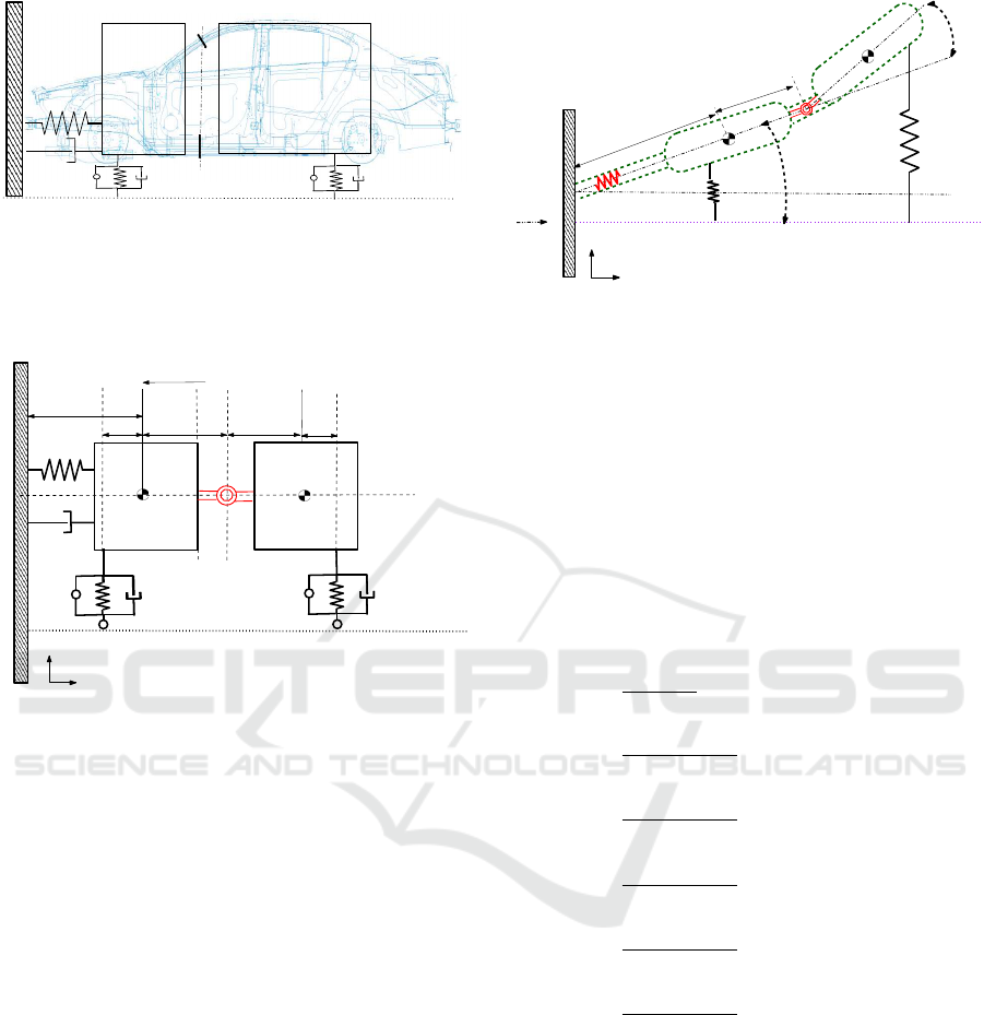
The motion of a double pendulum is described as
follows: the pendulum swings back and forth about
the pivot point as shown in Figure 1. Under impact,
the vehicle behaves like a pendulum rotating around
the pivot point, that is, an impact point in this case,
thus, causing the pitching. As a result of the ground
acting as a constraint, the vehicle cannot sway back
and forth. The deformable front end crumple zone is
represented with a spring and damper system for the
pendulum; the suspensions acting as a constraint to
prevent the pendulum to rotate beyond a certain an-
gle. The 3 Degrees of Freedom (DOF) LPM is de-
fined to determine the governing equations of motion;
the system is simplified by converting the cartesian
coordinates to polar coordinates.
Ground
Double Pendulum motion
θ
1
θ
1
θ
2
θ
2
Figure 1: Vehicle body rotating like a pendulum about the
impact point.
Figure 2 shows the model of the vehicle impact-
ing a rigid barrier. The front end deformation is
represented by the elastic pendulum; the spring and
damper coefficients are defined using a piecewise lin-
ear function with five breakpoints. The torsional
spring connects the mass components before and af-
ter the welded zone.The LPM containing two mass
Modeling of Modified Vehicle Crashworthiness using a Double Compound Pendulum
103

m
1
m
2
welds
k
1
c
1
k
1
c
1
Figure 2: Vehicle body with welds and the occupant com-
partments divided into lumped mass systems.
components along with the constraints is presented in
Figure 3
l
3
k
1
k
2
c
1
c
2
c
comp
k
comp
l
0
m
2
CG
Rigid Barrier
velocity = v
Ground
z
z
CG
m
1
k
tor
l
2
l
4
l
1
c
tor
dimensionless torsional spring
x
z
Figure 3: LPM of the vehicle impacting the rigid barrier at
time t = 0.
The event has been divided into three phases:
• Deformation of the front end leading to energy ab-
sorption modeled as an elastic spring.
• Rotation of the vehicle body about the impact
point with an angle θ
1
.
• Failure of the welds leading to rotation of the ve-
hicle about the torsional joint with an angle θ
2
.
The double pendulum model replicating the vehicle
rotating about the torsional spring with an angle θ
2
is
shown in Figure 4.
2.1 Parameter Identification for Front
End Spring and Damper
Characteristics
The front end spring damper characteristics were de-
fined using an algorithm developed by the authors
(Noorsumar et al., 2021b). The gradient descent opti-
mization algorithm has been modified to fit the force-
deformation curve for the entire dynamic event.
The spring and damper coefficients derived from
the algorithm are presented in the next section. The
Occupant compartment
Front deformed members
Torsional spring
θ
1
θ
2
Ground
l
0
+ r
l
1
x
z
Rigid Barrier
Figure 4: Vehicle body rotating about the impact point after
front-end deformation.
non-linear force deformation curve have been approx-
imated to represent the front end system in the LPM.
The stiffness k and spring force F
k
are related by the
equation (1). Similarly, the damper coefficient c is
related to the damping force F
c
by the equation (2)
((Elkady and Elmarakbi, 2012), (Noorsumar et al.,
2021b)).
F
k
= k(x) · x, (1)
F
c
= c( ˙x) · ˙x, (2)
where
k(x) =













































(k
2
−k
1
)·| ˆx|
x
1
+ k
1
, for | ˆx| ≤ x
1
,
(k
3
−k
2
)·(| ˆx|−x
1
)
(x
2
−x
1
)
+ k
2
, for x
1
≤ | ˆx| ≤ x
2
,
(k
4
−k
3
)·(| ˆx|−x
2
)
(x
3
−x
2
)
+ k
3
, for x
2
≤ | ˆx| ≤ x
3
,
(k
5
−k
4
)·(| ˆx|−x
3
)
(x
4
−x
3
)
+ k
4
, for x
3
≤ | ˆx| ≤ x
4
,
(k
6
−k
5
)·(| ˆx|−x
4
)
(x
5
−x
4
)
+ k
5
, for x
4
≤ | ˆx| ≤ x
5
,
(k
7
−k
6
)·(| ˆx|−x
5
)
(C−x
5
)
+ k
6
, for x
5
≤ | ˆx| ≤ C.
The damper characteristics are defined similar to the
spring characteristics in the model:
SIMULTECH 2022 - 12th International Conference on Simulation and Modeling Methodologies, Technologies and Applications
104

c( ˙x) =















































(c
2
−c
1
)·|
ˆ
˙x|
˙x
1
+ c
1
, for |
ˆ
˙x| ≤ ˙x
1
,
(c
3
−c
2
)·(|
ˆ
˙x|− ˙x
1
)
( ˙x
2
− ˙x
1
)
+ c
2
, for ˙x
1
≤ |
ˆ
˙x| ≤ ˙x
2
,
(c
4
−c
3
)·(|
ˆ
˙x|− ˙x
2
)
( ˙x
3
− ˙x
2
)
+ c
3
, for ˙x
2
≤ |
ˆ
˙x| ≤ ˙x
3
,
(c
5
−c
4
)·(|
ˆ
˙x|− ˙x
3
)
( ˙x
4
− ˙x
3
)
+ c
4
, for ˙x
3
≤ |
ˆ
˙x| ≤ ˙x
4
,
(c
6
−c
5
)·(|
ˆ
˙x|− ˙x
4
)
( ˙x
5
− ˙x
4
)
+ c
5
, for ˙x
4
≤ |
ˆ
˙x| ≤ ˙x
5
,
(c
7
−c
6
)·(|
ˆ
˙x|− ˙x
5
)
(v
0
− ˙x
5
)
+ c
6
, for ˙x
5
≤ |
ˆ
˙x| ≤ v
0
,
where k is the front end spring coefficient, c is the
front end damper coefficient, ˆx is the computed vehi-
cle deformation, ˙x is the vehicle velocity,
ˆ
˙x is the com-
puted vehicle velocity, C is the maximum dynamic
crush, v
0
is the velocity at the time of maximum dy-
namic crush. The optimization algorithm which mini-
mizes the error between the test and computed values
has been used to determine the acceleration, veloc-
ity and deformation of the vehicle (Noorsumar et al.,
2021b).
2.2 Defining the Equations of Motion
The governing equations of motion have been mod-
eled using the relativistic Lagrangian formulation
(Goldstein et al., 2002).
d
dt
∂L
∂ ˙q
i
−
∂L
∂q
i
+
∂D
∂q
i
= Q
i
, (3)
where, in general case, L = T −V, T is the total kinetic
energy of the system equal to the sum of the kinetic
energies of the particles, q
i
,i = 1,...,n are general-
ized coordinates and V is the potential energy of the
system. Here D is the dissipation function and Q
i
is
the external force acting on the system; in this case
it is the vertical component of the force experienced
by the vehicle at the time of maximum dynamic crush
(Noorsumar et al., 2021a).
The cartesian system is converted to polar coordi-
nates; the horizontal and vertical coordinates for the
two mass system (x
1
,y
1
) and (x
2
,y
2
) and the rotations
(θ
1
and θ
2
) about the y-axis have been represented in
(4)-(7):
x
1
= [l
0
+ r(t)]cosθ
1
(t), (4)
z
1
= [l
0
+ r(t)]sinθ
1
(t), (5)
x
2
=[l
0
+ r(t)]cosθ
1
(t) + l
1
cosθ
1
(t)
+ l
2
cosθ
2
(t),
(6)
z
2
=[l
0
+ r(t)]sinθ
1
(t) + l
1
sinθ
1
(t)
+ l
2
sinθ
2
(t),
(7)
where l
0
is the distance from the center of gravity
(CG) of mass m
1
to the point of impact of the ve-
hicle in the rest position, l
1
is the distance from the
CG
m1
to the front suspension, l
2
is the distance from
the CG
m2
to the rear suspension, r(t) is the displace-
ment along the polar radius of the elastic pendulum
spring, t is the time, and r, θ
1
and θ
2
are the radius
and angles in polar coordinates respectively. Taking
the derivatives with respect to time of x
1
, x
2
and z
1
, z
2
we obtain (8)-(11):
˙x
1
= ˙r cos θ
1
− (l
0
+ r)sin θ
1
·
˙
θ
1
,
(8)
˙z
1
= ˙r sin θ
1
+ (l
0
+ r)cos θ
1
·
˙
θ
1
,
(9)
˙x
2
=˙r cosθ
1
− (l
0
+ r)sin θ
1
·
˙
θ
1
− l
1
˙
θ
1
sinθ
1
− l
2
˙
θ
2
sinθ
2
,
(10)
˙z
2
=˙r sinθ
1
+ (l
0
+ r)cos θ
1
·
˙
θ
1
− l
1
˙
θ
1
sinθ
1
− l
2
˙
θ
2
sinθ
2
,
(11)
where ˙x
1
, ˙x
2
, ˙z
1
and ˙z
2
represent the velocity of the
mass components in horizontal and vertical direc-
tions. Squaring both sides of the equations gives
˙x
1
2
=˙r
2
cos
2
θ
1
+ (l
0
+ r)
2
sin
2
θ
1
·
˙
θ
1
2
− 2˙r cos θ
1
· (l
0
+ r)sin θ
1
·
˙
θ
1
,
(12)
˙z
1
2
=˙r
2
sin
2
θ
1
+ (l
0
+ r)
2
cos
2
θ
1
·
˙
θ
1
2
+ 2˙r cos θ
1
· (l
0
+ r)sin θ
1
·
˙
θ
1
,
(13)
˙x
2
2
= ˙x
1
2
+ l
2
1
˙
θ
1
2
sinθ
1
2
+ l
2
2
˙
θ
2
2
sinθ
2
2
− 2 ˙x
1
l
1
˙
θ
1
sinθ
1
+ 2l
1
l
2
˙
θ
1
˙
θ
2
sinθ
1
sinθ
2
− 2 ˙x
1
l
2
˙
θ
2
sinθ
2
,
(14)
˙z
2
2
= ˙z
1
2
+ l
2
1
˙
θ
1
2
cos
2
θ
1
+ l
2
2
˙
θ
2
2
cos
2
θ
2
+ 2l
1
l
2
˙
θ
1
˙
θ
2
cosθ
1
cosθ
2
+ 2 ˙z
1
l
1
˙
θ
1
cosθ
1
+ 2 ˙z
2
l
2
˙
θ
2
cosθ
2
.
(15)
Adding the terms we have:
˙x
1
2
+ ˙z
1
2
=˙r
2
(cos
2
θ
1
+ sin
2
θ
1
)
+ (l
0
+ r)
2
·
˙
θ
1
2
(cos
2
θ
1
+ sin
2
θ
1
),
(16)
˙x
2
2
+ ˙z
2
2
=x
1
2
+ x
2
2
+ l
2
1
˙
θ
1
2
+ l
2
2
˙
θ
2
2
− 2 ˙x
1
l
1
˙
θ
1
sinθ
1
+ 2l
1
l
2
˙
θ
1
˙
θ
2
sinθ
1
sinθ
2
− 2 ˙x
1
l
2
˙
θ
2
sinθ
2
+ 2 ˙z
1
l
1
˙
θ
1
cosθ
1
+ 2l
1
l
2
˙
θ
1
˙
θ
2
cosθ
1
cosθ
2
+ 2 ˙z
1
l
1
˙
θ
1
cosθ
1
+ 2 ˙z
1
l
2
˙
θ
2
cosθ
2
.
(17)
The kinetic energy of the system is given by
T =
1
2
[m
1
( ˙x
1
2
+ ˙z
1
2
) + m
2
( ˙x
2
2
+ ˙z
2
2
)],
(18)
Modeling of Modified Vehicle Crashworthiness using a Double Compound Pendulum
105

or, in polar coordinates,
T =
1
2
m
1
[˙r
2
+ (l
0
+ r)
2
˙
θ
1
2
]
+
1
2
m
2
[[˙r
2
+ (l
0
+ r)
2
·
˙
θ
1
2
+ l
2
1
·
˙
θ
1
2
+ l
2
2
·
˙
θ
1
2
]
+ 2l
1
l
2
˙
θ
1
˙
θ
2
sinθ
1
sinθ
2
− 2[˙r cos θ
1
− (l
0
+ r)
˙
θ
1
sinθ
1
]l
1
˙
θ
1
sinθ
1
]
− 2[˙r cos θ
1
− (l
0
+ r)
˙
θ
1
sinθ
1
]l
2
˙
θ
2
sinθ
2
].
(19)
The potential energy of the system can be found as
V =m
1
g(l
0
+ r)sin θ
1
+ m
2
g[(l
0
+ r)sin θ
1
+ l
1
sinθ
1
+ l
2
sinθ
2
]
+
1
2
k
comp
r
2
1
+
1
2
k
tor
θ
2
2
+
1
2
k
1
r
2
+
1
2
k
2
r
2
2
(20)
where r
1
and r
2
are expressed in terms of r, θ
1
, θ
2
, l
1
,
l
2
, l
3
as follows:
r
1
= (l
0
+ r −l
3
)θ
1
, (21)
r
2
= (l
0
+ r +l
1
)θ
1
+ l
2
θ
2
. (22)
Here m
1
is the mass of the lumped body before the
weld and HAZ, m
2
is the mass of the occupant com-
partment after the weld and HAZ, l
3
is the distance
from the CG
m1
to the front suspension, l
2
is the dis-
tance from the weld to the CG
m2
. Simplifying the
expression for potential energy in equation (20), we
obtain:
V =m
1
g(l
0
+ r)sin θ
1
+ m
2
g[(l
0
+ r)sin θ
1
+ l
1
sinθ
1
+ l
2
sinθ
2
]
+
1
2
k
1
(l
0
+ r − l
3
)
2
θ
2
+
1
2
k
2
((l
0
+ r + l
1
)θ
1
+ l
2
θ
2
)
2
+
1
2
k
comp
r
2
1
+
1
2
k
tor
θ
2
2
.
(23)
Here k
1
and k
2
are the suspension spring coefficients
for the front and rear suspensions respectively. Using
equations (19) and (23) and Lagrangian formulation,
L = T −V , we conclude that
L =
1
2
m
1
[˙r
2
+ (l
0
+ r)
2
˙
θ
1
2
] +
1
2
m
2
[˙r
2
+ (l
0
+ r)
2
˙
θ
2
2
+ l
1
˙
θ
1
2
+ l
2
˙
θ
2
2
− 2˙r
˙
θ
1
l
1
θ
1
+ 2(l
0
+ r)l
1
˙
θ
1
2
θ
2
1
+ 2l
1
l
2
˙
θ
1
˙
θ
2
θ
1
θ
2
− 2˙r
˙
θ
2
l
2
θ
2
+ 2l
2
(l
0
+ r)
˙
θ
1
˙
θ
2
θ
1
θ
2
]
− m
1
g(l
0
+ r)sin θ
1
− m
2
g[(l
0
+ r)sin θ
1
+ l
1
sinθ
1
+ l
2
sinθ
2
]
−
1
2
k
comp
r
2
1
−
1
2
k
tor
θ
2
2
−
1
2
k
1
r
2
−
1
2
k
2
r
2
2
,
(24)
The governing equations of motion are:
Q
ext
r
=m
1
¨r + m
2
¨r − m
2
l
1
(
¨
θ
1
θ
1
+ 2
˙
θ
1
)
− m
2
l
2
(
¨
θ
2
θ
2
+ 2
˙
θ
2
) − m
1
(l
0
+ r)
˙
θ
1
2
+ m
2
(l
0
+ r)
˙
θ
1
2
+ m
2
l
1
˙
θ
1
2
θ
2
1
+ m
2
l
2
˙
θ
1
˙
θ
2
θ
1
θ
2
+ m
1
gθ
1
+ m
2
gθ
2
+ k
01
(l
0
+ r − l
3
)θ
2
1
+ k
02
[(l
0
+ r + l
1
)θ
2
1
+ l
2
θ
1
θ
2
] + k
comp
r,
(25)
Q
ext
θ
1
=m
1
(l
0
+ r)
2
¨
θ
1
+ 2m
1
(l
0
+ r)˙r
˙
θ
1
+ 2m
2
(l
0
+ r)˙r
˙
θ
1
+ m
2
l
2
1
¨
θ
1
− m
2
l
1
˙
θ
1
˙r
− m
2
l
1
˙
θ
1
¨r + 2m
2
l
1
[˙r
˙
θ
1
θ
2
1
+ (l
0
+ r)θ
2
1
¨
θ
1
]
+ 2(l
0
+ r)l
1
˙
θ
1
2
θ
1
+ m
2
l
1
l
2
[
¨
θ
2
¨
θ
1
θ
2
+
˙
θ
2
˙
θ
1
θ
2
]
+ m
2
l
2
[˙r
˙
θ
2
θ
1
θ
2
+ (l
0
+ r)
¨
θ
2
θ
1
θ
2
+ (l
0
+ r)
˙
θ
2
˙
θ
1
θ
2
] + m
2
˙r
˙
θ
1
l
1
− 2m
2
(l
0
+ r)l
2
˙
θ
1
2
θ
1
− m
2
l
1
l
2
˙
θ
2
θ
1
θ
2
+ m
2
l
2
(l
0
+ r)
˙
θ
2
θ
1
θ
2
+ m
1
g(l
0
+ r) + m
2
g[(l
0
+ r) + l
1
]
− k
01
[l
0
+ r − l
3
]
2
θ
1
− k
02
[l
0
+ r + l
1
]
2
θ
1
− k
02
[l
0
+ r + l
1
]l
2
θ
2
,
(26)
Q
ext
θ
2
=m
2
l
2
2
¨
θ
2
+ m
2
l
1
l
2
[
¨
θ
1
θ
1
θ
2
+
˙
θ
1
2
θ
2
+
˙
θ
1
θ
1
˙
θ
2
]
− m
2
l
2
[˙r
˙
θ
1
θ
1
θ
2
+ (l
0
+ r)
¨
θ
1
θ
1
θ
2
+ (l
0
+ r)
˙
θ
1
2
θ
2
]
− m
2
l
1
l
2
˙
θ
1
˙
θ
2
θ
1
+ m
2
˙r
˙
θ
2
l
2
− m
2
l
2
(l
0
+ r)
˙
θ
1
˙
θ
2
θ
1
+ m
2
gl
2
+ k
02
[(l
0
+ r + l
1
)l
2
θ
1
+ l
2
2
θ
2
]
+ k
r
θ
2
(27)
where Q
ext
r
, Q
ext
θ
2
and Q
ext
θ
2
are the external forces act-
ing on the vehicle. The non-conservative forces in
the system are included in the Lagrange’s equation of
motion in the form of generalized forces expressed
with the formulation of virtual work δU (Cyr
´
en and
Johansson, 2018):
δU =
m
∑
j=1
F
j
· δr
j
(28)
where F
j
are the force components, δr
j
are the virtual
displacements given by
δr
j
=
N
∑
i=1
∂r
j
∂q
i
δq
i
(29)
for j = 1,2,3, . ..,m. This yields the following equa-
tion for virtual work:
δU = F
1
·
N
∑
i=1
∂r
j
∂q
i
δq
i
+ F
2
·
N
∑
i=1
∂r
j
∂q
i
δq
i
+ · · ·
+F
m
·
N
∑
i=1
∂r
j
∂q
i
δq
i
.
(30)
Using equation (30), we compute the generalized
SIMULTECH 2022 - 12th International Conference on Simulation and Modeling Methodologies, Technologies and Applications
106

forces acting the system:
δU = F
x
1
·

∂x
∂r
· δr +
∂x
∂θ
1
· δθ
1
+
∂x
∂θ
2
· δθ
2

+F
x
2
·

∂x
∂r
· δr +
∂x
∂θ
1
· δθ
1
+
∂x
∂θ
2
· δθ
2

+F
z
1
·

∂z
∂r
· δr +
∂z
∂θ
1
· δθ
1
+
∂z
∂θ
2
· δθ
2

+F
z
2
·

∂z
∂r
· δr +
∂z
∂θ
1
· δθ
1
+
∂z
∂θ
2
· δθ
2

.
(31)
Substituting equations (4) and (5) in equation (31), we
get
dU = F
x
1
· [(cos(θ
1
)δr − (l
0
+ r)sin θ
1
δθ
1
]
+F
x
2
· [(cos(θ
1
)δr − (l
0
+ r)sin θ
1
δθ
1
− l
1
sinθ
1
δθ
1
−l
2
sinθ
2
δθ
2
] + F
z
1
· [(sin(θ
1
)δr + (l
0
+ r)cos(θ
1
)δθ
1
]
+F
z
2
· [(sin(θ
1
)δr + (l
0
+ r)cos(θ
1
)δθ
1
+ l
1
cosθ
1
δθ
1
+l
2
cosθ
2
δθ
2
].
(32)
The external forces included in this LPM are bar-
rier forces, damper forces including front end spring
damper system and suspension damper system forces.
The corresponding equations are:
Q
ext
r
= Q
bar
r
+ Q
damp
r
, (33)
Q
ext
θ
1
= Q
bar
θ
1
+ Q
damp
θ
1
, (34)
Q
ext
θ
2
= Q
bar
θ
2
+ Q
damp
θ
2
. (35)
Here F
x
and F
z
are the horizontal and vertical force
components acting on the vehicle; Q
bar
r
, Q
damp
θ
1
and
Q
damp
θ
2
are the non-conservative barrier and damper
forces acting on the system.
Then δU assumes the form
δU = Q
damp
r
· δr +Q
damp
θ
1
· δθ
1
+ Q
damp
θ
2
· δθ
2
+Q
bar
r
· δr +Q
bar
θ
1
· δθ
1
+ Q
bar
θ
2
· δθ
2
(36)
where
Q
bar
r
=F
bx
1
cosθ
1
+ F
bz
1
sinθ
1
+ F
bx
2
cosθ
1
+ F
bz
2
sinθ
1
,
(37)
Q
bar
θ
1
= − F
bx
1
(l
0
+ r)sin θ
1
+ F
bz
1
(l
0
+ r)cos θ
1
− F
bx
2
[(l
0
+ r)sin θ
1
+ l
1
sinθ
1
]
+ F
bz
2
[(l
0
+ r)cos θ
1
+ l
1
cosθ
1
],
(38)
Q
bar
θ
2
= −F
bx
2
l
2
sinθ
2
+ F
bz
2
l
2
cosθ
2
(39)
where F
bx
and F
bz
are the barrier forces acting on
the vehicle in the horizontal and vertical directions.
These values are included from the FE simulation
data. The derivative of the dissipation energy D and
the damper forces are given by the equations
D =
1
2
c
comp
˙r
2
+
1
2
c
1
[(l
0
+ r −l
3
)
˙
θ
1
+ ˙rθ
1
]
2
+
1
2
c
2
[(l
0
+ r +l
1
)
˙
θ
1
+ ˙rθ
1
+ l
2
θ
2
]
2
+
1
2
c
tor
˙
θ
2
,
(40)
Q
damp
r
=F
bx
1
cosθ
1
+ F
bz
1
sinθ
1
+ F
bx
2
cosθ
1
+ F
bz
2
sinθ
1
,
(41)
Q
damp
θ
1
= − F
bx
1
(l
0
+ r)sin θ
1
+ F
bz
1
(l
0
+ r)cos θ
1
− F
bx
2
[(l
0
+ r)sin θ
1
+ l
1
sinθ
1
]
+ F
bz
2
[(l
0
+ r)cos θ
1
+ l
1
cosθ
1
],
(42)
Q
damp
θ
2
= −F
bx
2
l
2
sinθ
2
+ F
bz
2
l
2
cosθ
2
,
(43)
where c
1
and c
2
are the damper coefficients for the
front and rear suspensions, c
comp
and c
tor
are the
damper coefficients from the front end compression
spring and the torsional spring respectively.
2.3 Validation with an FE Model
The LPM is validated against a modified FEM devel-
oped by NHTSA (NHTSA, 2017) where the effect of
welding and material behavioural changes in UHSS
structural members is included by the authors. The
crashworthiness response is affected by the changes
in material behaviour which compromise the safety
performance. The acceleration, velocity and displace-
ment curves from the 2010 Toyota Yaris FE model
for a full frontal impact were used to validate the
LPM performance. The speed of the impact was 56
kmph and the barrier is a rigid non deformable bar-
rier with 0% offset. The baseline FE model devel-
oped by National Crash Analysis Center (NCAC) and
National Highway Transport Safety Administration
(NHTSA) (Marzougui et al., 2011), (NHTSA, 2017)
was adopted to modify the structural members. The
model is cut and welded to incorporate the repairs of
UHSS material on load bearing structural members.
The material and section properties of the weld were
adopted from a similar FE developed in (Noorsumar
et al., 2020). The weld zone and HAZ lead to reduced
strength in the members and replicates the behaviour
in a physical test. It will be interesting to use physical
test data in a future study.
Figure 5 shows the FE model developed by
NHTSA which replicates a 2010 four-door passenger
sedan consisting of 917 parts, 1,480,422 nodes and
1,514,068 elements. The FE model weighs 1,100 kg
which is close to the physical test vehicle weighing
Modeling of Modified Vehicle Crashworthiness using a Double Compound Pendulum
107

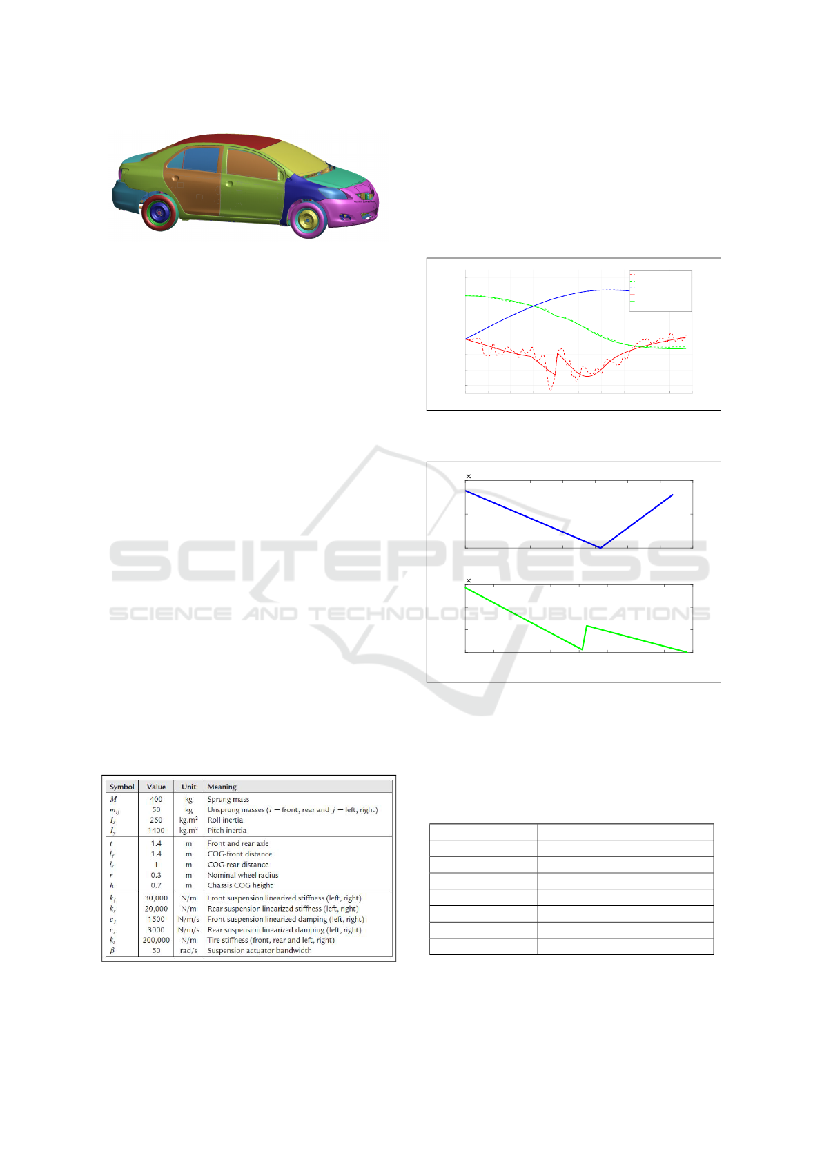
Figure 5: Baseline 2010 Toyota Yaris FE Model.
1,078 kg.The model was correlated with a number of
crash loadcases confirming the reliability of the model
representing the physical vehicle.
The next section highlights the results and discus-
sion on the model simulations.
3 RESULTS AND DISCUSSION
The LPM defined in the Section 2 was simulated in
MATLAB Simulink and the results were compared
with the data generated from the LS Dyna FE model
for a 2010 Toyota Yaris impacting a rigid barrier at
56 kmph. Prior to overlaying the LS Dyna curve out-
puts with the LPM results, the FE outputs were con-
verted into polar coordinates to compare the results.
The Simulink model was run with an ode45 (variable
timestep) solver; it was observed that changing the
solver parameters did not influence the results signif-
icantly. The maximum values of the pitching angles
θ
1
and θ
2
are crucial to determine the occupant in-
jury prediction during the vehicle development stage.
The maximum crush of the vehicle and the velocity
during energy absorption stage helps predict the vehi-
cle crashworthiness performance in an impact. These
parameters have been measured with the Simulink
model developed in the study. The values of k
1
, k
2
,
c
1
, c
2
have been adopted from (Savaresi et al., 2010)
and presented in Table 1.
Table 1: Automotive Parameters set (Savaresi et al., 2010).
The front-end spring and damper coefficients
(k
comp
and c
comp
) were determined from the optimiza-
tion algorithm presented in Subsection 2.1. The LPM
was compared against the data from FE in the param-
eter identification code. The computed acceleration,
velocity and displacement curves are shown in Figure
6. The corresponding spring and damper coefficients
are presented in Figure 7.
0 0.01 0.02 0.03 0.04 0.05 0.06 0.07 0.08 0.09 0.1
t [s]
-60
-40
-20
0
20
40
60
80
a [g], v[km/h], s [cm]
Result and Comparison, non-linear damper and spring
FE Data - acceleration
FE Data - velocity
FE Data - displacement
LPM - acceleration
LPM - velocity
LPM - displacement
Figure 6: Comparison of FE and LPM curves for parameter
identification algorithm.
0 0.1 0.2 0.3 0.4 0.5 0.6 0.7
displacement [m]
0
5
10
Spring coeff [N/m]
10
5
Spring coefficient
0 2 4 6 8 10 12 14 16
velocity [m/s]
0
5
10
15
Damper coeff [Ns/m]
10
4
Figure 7: Front-end Spring and Damper coefficients for
Toyota Yaris.
The values of m
1
, m
2
, l
0
,l
1
, l
2
, l
3
, k
tor
, c
tor
along
with external forces F
bx
1
, F
bz
1
, F
bx
2
, F
bz
2
were calcu-
lated from the LS Dyna model and presented in Table
2.
Table 2: Model Parameters.
Mass Body 1 m
1
539 kg
Mass Body 2 m
1
629 kg
l
1
0.57 (metres)
l
2
1.3 (metres)
l
3
0.10 (metres)
l
0
0.91 (metres)
k
tors
Curves from LS Dyna model
c
tors
Curves from LS Dyna model
Figure 8 shows the change in the velocity of the
vehicle in m/s after the impact. The LPM was over-
SIMULTECH 2022 - 12th International Conference on Simulation and Modeling Methodologies, Technologies and Applications
108

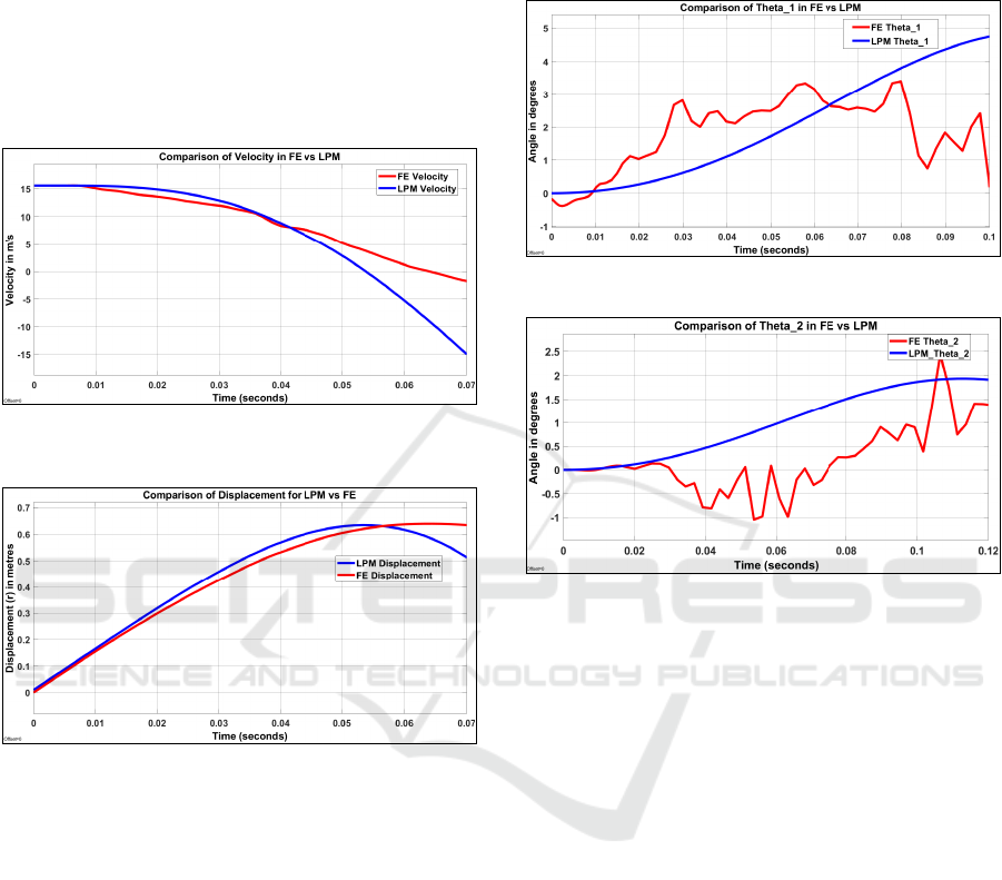
laid with the FE data curves and the plots show good
correlation of the time when the vehicle attains zero
velocity. The trend of the curves is similar indicating
the impact kinematics has been replicated in the LPM.
The maximum deformation experienced by the vehi-
cle during the full frontal impact is shown in Figure
9 and the maximum crush values are closely corre-
lated, demonstrating a good prediction capability of
the model.
Figure 8: Velocity of the vehicle - curves comparison for
LPM vs FE model.
Figure 9: Displacement of the vehicle front-end - curves
comparison for LPM vs FE model.
Figure 10 shows the plot of θ
1
which indicates the
pitching of the vehicle about the point of impact. The
curves for the LPM over-predict the maximum pitch-
ing angle; this could be attributed to the approxima-
tion of the model parameters like suspension spring
and damper coefficients which were assumed to be
constant throughout the simulation. It is however, cru-
cial to predict the maximum pitching angle to design
the restraint systems for occupants in the vehicle; the
pitching angle θ
1
is closely correlated in the LPM de-
veloped in this study.
As explained in Section 2, the model uses a tor-
sional spring to represent fractures in the structural
members due to HAZ (from welding or heat treat-
ment processes); leading to an angle θ
2
in the vehicle
pitching. The plot for θ
2
is shown in Figure 11; the
stiffness of the spring is approximated from the weld
failure data used in the FE model. It is observed that
the predicted angle from the LPM is close to the max-
imum value from the FE model, however, the model
can be further improved.
Figure 10: θ
1
curve comparison for LPM vs FE model.
Figure 11: θ
2
curve comparison for LPM vs FE model.
4 CONCLUSIONS AND NEXT
STEPS
The reliability of mathematical modeling to replicate
and predict vehicle crashworthiness response has in-
creased during the last decade. These models are
slowly replacing physical tests; LPMs provide results
with low computational time and fewer vehicle pa-
rameters. LPMs can be used during the initial stages
of the vehicle development process when full scale
CAD models are not available. The literature re-
view indicated little research in the area of represent-
ing welds and material failure in LPMs. Our 3 DOF
LPM predicts the following vehicle parameters in a
full frontal impact:
• Maximum vehicle crush during an impact.
• Time for the vehicle to reach zero velocity from
the start of the event.
• Vehicle pitching angle about the point of impact.
• Failure of the structural members leading to
higher pitching angle in a modified vehicle.
The model uses an elastic double compound pendu-
lum replicating the event kinematics to capture the
Modeling of Modified Vehicle Crashworthiness using a Double Compound Pendulum
109

front-end deformation and the rotation of the vehicle;
first around the point of impact and then around the
failure of the material due to welding or heat treat-
ment. The LPM employs Lagrangian formulation to
define the equations of motion and is presented in po-
lar coordinates to simplify the system. The model cor-
relates well with the FE data for a 2010 Toyota Yaris;
the deformation, velocity and pitching angle are pre-
dicted well for a full frontal impact at 56 kmph. The
failure of the structural members is simulated in the
model with a torsional spring. The angle of rotation
of the vehicle θ
2
due to material behavioural changes
is close to the maximum values in the validation data.
The novel methodology presented in this study
can be further enhanced with real-time weld fracture
data from physical tests. The model predictability can
be further improved by replacing the piece-wise linear
approximation for the vehicle parameter values with
non-linear functions for stiffness and damping coeffi-
cients.
ACKNOWLEDGEMENTS
The authors would like to thank Top Research Center
Mechatronics (TRCM) at University of Agder for the
support to conduct the research. We would also like
to acknowledge the support of NHTSA and NCAC for
the FE models used in this study.
REFERENCES
Amirthalingam, M., Hermans, M., and Richardson, I.
(2009). Microstructural development during weld-
ing of siliconand aluminum-based transformation-
induced plasticity steels-inclusion and elemental par-
titioning analysis. Metallurgical and Materials Trans-
actions A: Physical Metallurgy and Materials Sci-
ence, 40(4):901–909.
Benson, D., Hallquist, J., Igarashi, M., Shimomaki, K., and
Mizuno, M. (1986). Application of DYNA3D in large
scale crashworthiness calculations.
B
¨
ottcher, C. S., Frik, S., and Gosolits, B. (2005). 20 years of
crash simulation at Opel-experiences for future chal-
lenges. 4th LS-DYNA Anwenderforum, pages 79–86.
Chang, J. M., Ali, M., Craig, R., Tyan, T., El-Bkaily, M.,
and Cheng, J. (2006a). Important modeling practices
in CAE simulation for vehicle pitch and drop. In SAE
Technical Papers. SAE International.
Chang, J. M., Huang, M., Tyan, T., Li, G., and Gu, L.
(2006b). Structural optimization for vehicle pitch and
drop. In SAE Technical Papers. SAE International.
Cyr
´
en, O. and Johansson, S. (2018). Modeling of Occupant
Kinematic Response in Pre-crash Maneuvers A sim-
plified human 3D-model for simulation of occupant
kinematics in maneuvers.
Elkady, M. and Elmarakbi, A. (2012). Modelling and anal-
ysis of vehicle crash system integrated with different
VDCS under high speed impacts. Central European
Journal of Engineering, 2(4):585–602.
Elkady, M., Elmarakbi, A., and Macintyre, J. (2012). En-
hancement of vehicle safety and improving vehicle
yaw behaviour due to offset collision using vehicle
dynamics. International Journal of Vehicle Safety,
6(2):110–133.
Goldstein, H., Poole, C., Safko, J., and Addison, S. R.
(2002). Classical Mechanics, 3rd ed. American Jour-
nal of Physics, 70(7):782–783.
Ionut, R. A., Corneliu, C., and Bogdan, T. (2017). Math-
ematical model validated by a crash test for study-
ing the occupant’s kinematics and dynamics in a cars’
frontal collision. International Journal of Automotive
Technology 2017 18:6, 18(6):1017–1025.
Kamal, M. M. (1970). Analysis and simulation of vehicle
to barrier impact. SAE Technical Papers, pages 1498–
1503.
Marzougui, D., Brown, D., Park, H. K., Kan, C. D., and
Opiela, K. S. (2011). 3 th International LS-DYNA
Users Conference Session: Automotive Development
& Validation of a Finite Element Model for a Mid-
Sized Passenger Sedan.
Mentzer, S. G., Radwan, R. A., and Hollowell, W. T. (1992).
The SISAME methodology for extraction of optimal
lumped parameter structural crash models. SAE Tech-
nical Papers.
NHTSA (2017). Crash simulation vehicle models.
Noorsumar, G., Robbersmyr, K., Rogovchenko, S., and
Vysochinskiy, D. (2020). Crash Response of a Re-
paired Vehicle - Influence of Welding UHSS Mem-
bers. In WCX SAE World Congress Experience. SAE
International.
Noorsumar, G., Rogovchenko, S., Robbersmyr, K., and
Vysochinskiy, D. (2021a). Mathematical models for
assessment of vehicle crashworthiness: a review. In-
ternational Journal of Crashworthiness.
Noorsumar, G., Rogovchenko, S., Robbersmyr, K.,
Vysochinskiy, D., and Klausen, A. (2021b). A novel
technique for modeling vehicle crash using lumped
parameter models. In Proceedings of the 11th In-
ternational Conference on Simulation and Modeling
Methodologies, Technologies and Applications, SI-
MULTECH 2021.
Noorsumar, G., Vysochinskiy, D., Englund, E., Rob-
bersmyr, K. G., and Rogovchenko, S. (2021c). Ef-
fect of welding and heat treatment on the properties
of UHSS used in automotive industry. EPJ Web of
Conferences, 250:05015.
Pavlov, N. (2019). Study the vehicle pitch motion by spring
inverted pendulum model. (February).
Pifko, A. and Winter, R. (1981). Theory and Application of
Finite Element Analysis To Structural Crash Simula-
tion, volume 13. Pergamon Press Ltd.
Savaresi, S., Poussot-Vassal, C., Spelta, C., Sename, O., and
SIMULTECH 2022 - 12th International Conference on Simulation and Modeling Methodologies, Technologies and Applications
110

Dugard, L. (2010). Semi-Active Suspension Control
Design for Vehicles. Elsevier Ltd.
Subedi, D., Tyapin, I., and Hovland, G. (2020). Model-
ing and Analysis of Flexible Bodies Using Lumped
Parameter Method. In Proceedings of 2020 IEEE
11th International Conference on Mechanical and In-
telligent Manufacturing Technologies, ICMIMT 2020,
pages 161–166. Institute of Electrical and Electronics
Engineers Inc.
Sypniewska-Kami
´
nska, G., Starosta, R., and Awrejcewicz,
J. (2016). Double pendulum colliding with a rough
obstacle. In Dynamical Systems - Mechatronics
and Life Sciences. Instytut Mechaniki Stosowanej,
Wydział Budowy Maszyn i Zarza¸dzania, Politechnika
Pozna
´
nska.
Sypniewska-Kami
´
nska, G., Starosta, R., and Awrejcewicz,
J. (2017). Motion of double pendulum colliding
with an obstacle of rough surface. Arch Appl Mech,
87:841–852.
Zhang, M., Li, L., Fu, R. y., Zhang, J. c., and Wan, Z.
(2008). Weldability of Low Carbon Transformation
Induced Plasticity Steel. Journal of Iron and Steel Re-
search, International, 15(5):61–87.
Modeling of Modified Vehicle Crashworthiness using a Double Compound Pendulum
111