Analysis of Differential Algebraic Equation Systems for Connecting

Energy Storages of Generally Valid Functional Mock-up Units

Meik Ehlert

, Christian Henke

and Ansgar Trächtler

Fraunhofer Institute for Mechatronic Systems Design IEM, Zukunftsmeile 1, Paderborn, Germany

Heinz-Nixdorf-Institute, University of Paderborn, Fürstenallee 11, Paderborn, Germany

Keywords: FMI, FMU, DAE, Energy Storage, Multi Body System, Model Coupling, Co-simulation.

Abstract: Functional Mock-up Units (FMU) refer to tool-independent models exported from their original simulation

tools. They enable component manufacturers and system integrators to exchange models across entire

production chains to validate solutions virtually. However, since system equations cannot be accessed or

modified in an FMU, numerical challenges can arise, especially when coupling similar energy storages. In

this paper, therefore, Differential Algebraic Systems of Equations are analyzed for their suitability for FMU

couplings. It is shown how such systems of equations can be described in a general way and how suitable

coupling constraints for FMUs are chosen. Subsequently, three solution approaches are presented and

analyzed for their feasibility with FMUs.

1 INTRODUCTION

Due to the increasing complexity in mechatronic

systems, a continuous simulation in the development

is indispensable (Michael et al., 2016). In this way,

partial solutions can already be virtually validated in

domain-specific development. This reduces the

construction of necessary prototypes and thus leads to

increased cost and time efficiency.

However, a particular challenge lies in the large

number of interacting domains. Specialized tools are

often used for different domains. System integrators

must therefore couple models from a heterogeneous

tool landscape with each other in order to represent

the overall system. The Functional Mock-up Interface

(FMI) has proven to be a widely used way of coupling

models in a tool-independent manner. Models are

exported from their original modeling tools as

compiled binary files. These are called Functional

Mock-up Units (FMU). The models can then be

interconnected via a standardized interface.

In addition to the tool-independent coupling of the

models, the FMI standard also allows industrial

know-how protection to be achieved. Since the model

behavior is represented by binary files, the internal

https://orcid.org/0000-0002-3905-4407

https://orcid.org/0000-0001-7611-7983

https://orcid.org/0000-0001-9987-1655

system equations can no longer be accessed or

changed. Thus the FMI standard can be used for a

modular model exchange over entire production

chains. Manufacturers of individual components, e.g.

from the electrical drive technology, have the

opportunity to pass on models to customers without

disclosing their know-how. This increases market

visibility and enlarges the customer base. On the other

hand, system integrators can test components from

different manufacturers virtually in their overall

solution.

The model boundaries of an FMU can be defined

as small as desired. For example, an FMU can

represent a physical component or an entire assembly.

However, a component can also be divided further, so

that an FMU can also be created at subcomponent

level. For example, an industrial converter can be

divided into a rectifier and an inverter. Similarly,

individual FMUs can be created from software

components, such as control algorithms. A large

number of FMUs in the overall system ensures

greater modularization. Individual submodels can be

exchanged and reused more easily. For example, the

user can assemble his own system model from a set

of prefabricated FMUs.

Ehlert, M., Henke, C. and Trächtler, A.

Analysis of Differential Algebraic Equation Systems for Connecting Energy Storages of Generally Valid Functional Mock-up Units.

DOI: 10.5220/0011305700003274

In Proceedings of the 12th International Conference on Simulation and Modeling Methodologies, Technologies and Applications (SIMULTECH 2022), pages 311-318

ISBN: 978-989-758-578-4; ISSN: 2184-2841

311

However, the tighter the model boundaries are

chosen, the higher is the integration effort in the

overall system and numerical difficulties can occur.

This is especially the case when similar energy

storages are interconnected across model boundaries.

Energy storages are physical elements, such as

masses, springs, capacitances or inductances, whose

state is described by its stored energy. For example,

if two masses are rigidly coupled together, they have

the same state. However, if the two masses are

arranged in two different models, each model

calculates its own state for the masses, which are

independent of each other.

In this article, therefore, methods are analyzed

with which FMUs can be coupled to overall systems

in a generally valid way. Special attention is paid to

the representation of a total system as a differential

algebraic equation (DAE) system. The couplings

should be possible independently of the energy

storage distribution in the system, so that two similar

energy storages, which are arranged in different

FMUs, can be rigidly coupled. In this paper, masses

are considered as an example.

2 STATE OF THE ART

In the following, the required information about the

Functional Mock-up Interface is given. Subsequently,

methods for coupling two masses from conventional

modeling are presented. An evaluation is made

whether these methods can be implemented with the

FMI standard.

2.1 Functional Mock-up Interface

The Functional Mock-up Interface refers to a standard

agreed upon by various vendors of modeling and

simulation tools to export their models as binary files.

With this standard a Co-Simulation or a model

integration can be performed. The exported models

are called Functional Mock-up Units. The standard

was first published in 2011 and currently exists in

versions 1.0 and 2.0. In addition, a pre-release of

version 3.0 exists since 2021 (FMI Development

Group, 2014).

An FMU consists of two files, a DLL file and an

XML file. The DLL file is the binary file that

represents the model behavior. For this purpose, it

implements the system equations of a general

nonlinear system, as follows.

𝑥

𝑓



𝑥,𝑢,𝑡



(1)

𝑦𝑤



𝑥,𝑢,𝑡



(2)

With

 𝑥: System State

 𝑢: System Input

 𝑦: System Output

 𝑡: System Time

The DLL file offers functions to read and write

the variables. In addition, a single simulation step can

be executed. The equations 𝑓 and 𝑤, however, cannot

be accessed.

The XML file represents the model description,

which contains all the required model information. It

lists which variables the model contains. Value

references are specified for these variables, which can

be used for the model functions from the DLL file to

reference a variable. Other attributes that a variable

can have are variability and causality. Causality

specifies whether a variable is an input, output or

parameter. Variability specifies whether a variable

may be changed during the simulation. Possible

values here are fixed and tunable. For example, output

variables cannot be written by the user, but are only

calculated by the model (FMI Development Group,

2014).

In (Blochwitz et al., 2012) an approach was

presented to couple masses in different FMUs. For

this purpose, a function for calculating directional

derivatives is used, which was introduced in the FMI

2.0 version. This can be used to compute a Jacobian

matrix that can be used to solve algebraic loops

created by the coupling. However, for this approach,

the appropriate input and output variables for the

FMUs must be provided. In this approach, one mass

provides the position, velocity and acceleration as

output. The second mass uses these quantities as input

and calculates a counter torque as output. An example

is provided by the Standard Modelica Library in the

GenerationOfFMUs example. However, these

masses have different interfaces and are not

considered as generally valid in this article.

Furthermore, the determination of directional

derivatives refers only to the FMU inputs. Moreover,

this function is optional and is only implemented by

a few tools.

2.2 Coupling of Similar Energy

Storages

In this section, first the problems of coupling similar

energy storages are shown. Then, common

approaches for solving the problem are presented.

Table 1 summarizes the energy storages from the

SIMULTECH 2022 - 12th International Conference on Simulation and Modeling Methodologies, Technologies and Applications

312

mechanical and electrical domains and shows the

corresponding differential equations (Isermann,

2007). The input and output quantities given result

from the assumption that the equations are solved by

numerical integrations only.

Table 1: Equations of Energy Storages.

Energy

Storages

Equations Input Output

Inductor

𝚤

𝐿

∙𝑢

𝑢 𝑖

Capacitor

𝑢 

𝐶

∙𝑖

𝑖 𝑢

Mass

𝑣

𝑚

∙𝐹

𝐹 𝑣

Spring

𝐹



𝑐∙𝑥

𝑐∙𝑣

𝑣 𝐹

The following system variables appear in the

equations from Table 1:

 𝑢: voltage

 𝑖: current

 𝑣: velocity

 𝐹: force

The parameters of the energy storages are given as:

 𝐿: inductance

 𝐶: capacity

 𝑚: mass

 𝑐: spring stiffness

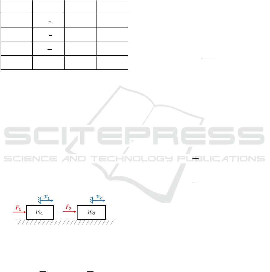
In this paper masses are considered for coupling

similar energy storages. In order to couple two

masses, they are first considered individually. Figure

1 shows a free cut of two masses 𝑚



and 𝑚



Figure 1: Free cut of two masses.

Each mass is driven by a force 𝐹, resulting in a

velocity 𝑣. The two masses are described by the

differential equations from table 1:

𝑣











𝐹



𝑣











𝐹



(3)

For each equation the input and output variables from

table 1 are given. Thus, each mass has the force 𝐹 as

input and the velocity 𝑣 as output. In this case the

problem with the coupling of two masses is obvious,

if they are located in different models. Both masses

expect a force as input. However, the first mass

provides a velocity as output, which cannot drive the

second mass. Thus, there is an interface

inconsistency. In (Ehlert et al., 2021) approaches

were presented with which energy storages can be

coupled, when all equations are known and

adjustable. These approaches are presented in the

following.

2.2.1 Substitute Variables

One of the most common methods for coupling

similar energy storages in conventional modeling is

the creation of substitute quantities. In this case, the

two masses are calculated to a total mass. This results

in a differential equation for both masses.

𝑣







𝐹 (4)

With this method, exact simulation results with a fast

computation time can be expected. However, the

system equations must be changed for this, which is

not possible with FMUs.

2.2.2 Fictitious Coupling Elements

Another possibility is the dynamic coupling via

fictitious coupling elements. In the case of two

masses, a fictitious spring is placed between the

masses. From this, the following differential

equations are derived:

𝑣











∙𝐹



𝐹



 (5)

𝐹





𝑐∙𝑣



𝑣



 (6)

𝑣











∙𝐹



𝐹



 (7)

Each mass is only dependent on its own input force

and the fictitious spring force 𝐹



. Thus, the states of

the masses are decoupled from each other. The stiffer

the spring is chosen, the more a rigid coupling is

approximated.

However, this approach can lead to long

computation times if the spring is chosen to be very

stiff, since this results in small time constants in the

system. On the other hand, if the stiffness is too small,

the simulation results are distorted by fictitious

dynamics.

One possibility to solve the coupled system with

less computational effort is to perform an order

reduction before the simulation. Equations (5) to (7)

represent a third order differential equation system.

Since a rigid coupling is approximated here, the

difference of the independent states 𝑣



and 𝑣



will be

very small. Here, an order reduction can compute a

minimum order in which no independent states for the

Analysis of Differential Algebraic Equation Systems for Connecting Energy Storages of Generally Valid Functional Mock-up Units

313

velocities would be considered. In the field of

snapshot-based methods, there exist procedures for

model order reduction that can also be implemented

as a black box (Benner et al., 2021). It will be

separately analyzed if these methods can be applied

to FMUs.

2.2.3 Definition of Coupling Constraints

A third way of coupling similar energy storages is to

define constraints. Thereby, the ordinary differential

equations of the masses are arranged independently in

a state space model. This is completed by coupling

constraints to a Differential Algebraic System (DAE).

In (Najafi, 2018), an extension of the Functional

Mock-up Interface is presented to solve DAE systems

in FMUs. In this approach, however, the algebraic

constraints are part of the FMUs. In this paper, the

constraints are formed by the coupling. Thus, they are

located outside the FMUs and have to be solved by a

higher-level simulation algorithm considering the

available model information.

Since the ordinary differential equations from the

FMUs are considered independently, this approach

will be further analyzed.

3 MODEL COUPLING USING

DAE-SYSTEMS

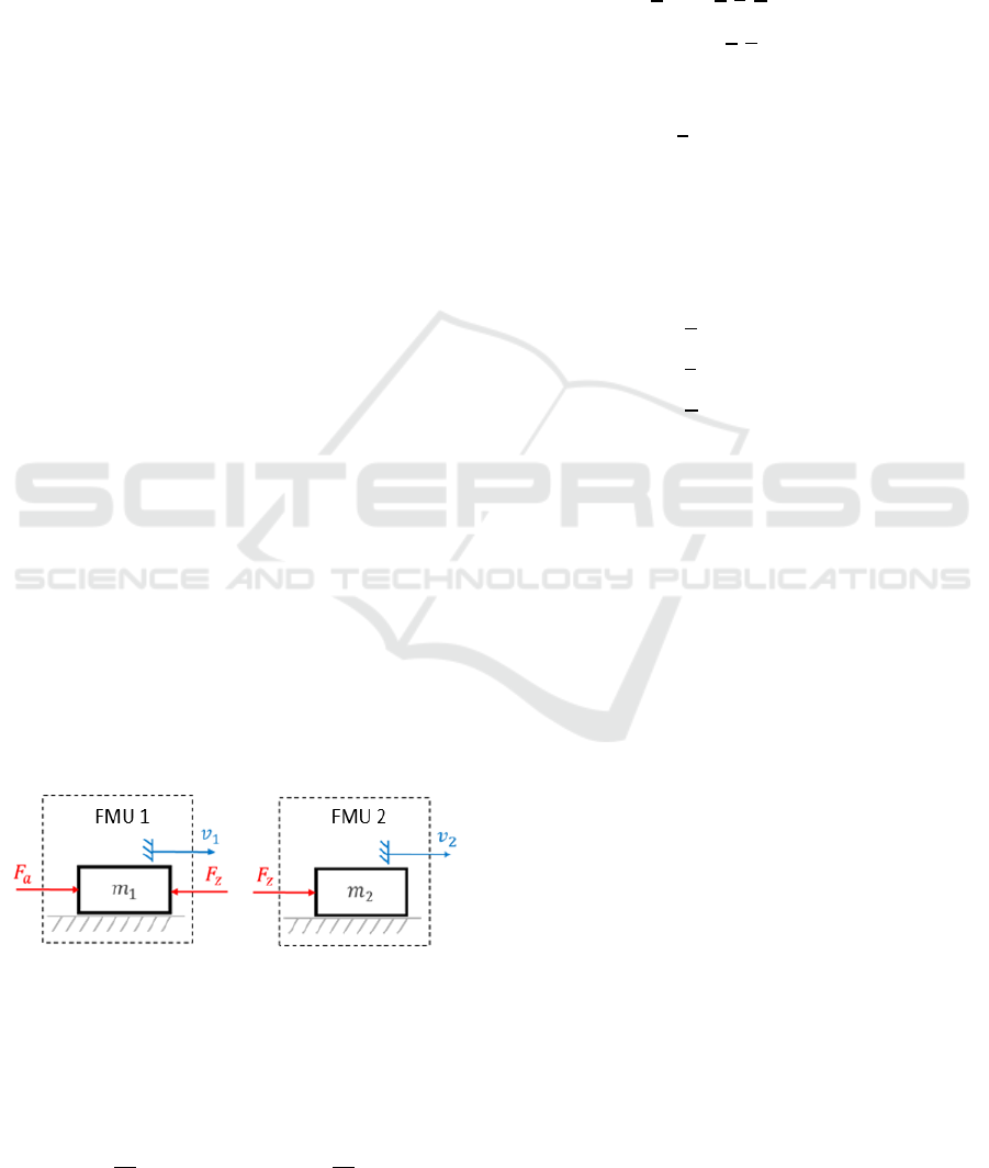
For the model coupling using DAE systems, two

masses are considered again. Each mass is arranged

in its own FMU, as shown in Figure 2. Both FMUs

have at least one force input and one velocity output.

The coupling is realized via a constraint force 𝐹



which can be applied via the force inputs in the

FMUs. In addition, the first mass is actuated via a

driving force 𝐹



Figure 2: Coupled masses using coupling constraints.

For the example shown, a DAE system can now be

set up. DAE systems consist of a set of ordinary

differential equations (ODE) and a set of algebraic

constraints. The ordinary differential equations for

the system shown above are:

𝑣











𝐹



𝐹



 𝑣











𝐹



(8)

Whereas an algebraic equation could limit the

velocities:

𝑣



𝑣



0

(9)

In general, DAE systems are defined as follows

(Janschek, 2010):

𝑥



𝑓



𝑥,𝑧,𝑢,𝑡



(10)

0𝑔



𝑥,𝑧,𝑡



(11)

Here, 𝑓 represents the set of ordinary differential

equations and 𝑔 the set of algebraic constraints. The

additional vector 𝑧

describes all algebraic variables

that do not occur differentially. It should be noted that

the DAE system represents the overall system and not

the individual FMUs. Therefore, the DAE system has

only the driving force 𝐹



as input and not the other

FMU inputs used for coupling. For the example

above, this results in the following assignments:

 𝑥





𝑣



,𝑣







(12)

 𝑧

𝐹



(13)

 𝑢

𝐹



(14)

In order to be able to couple models using DAE

systems, possible coupling constraints are analyzed

first. Then, the index of a DAE system has to be

determined in order to be able to select a solution

approach based on it.

3.1 Choice of Coupling Constraints

Coupling constraints can be chosen differently for

different systems. An example is provided by the

Modelica modeling language (Elmquist et al., 1998).

Here, the user creates a topology of a system. The

modeling tool that implements the Modelica language

uses this topology to create coupling constraints for

the basic differential equations of the modeling

modules and thus generates a system of equations.

The coupling constraints are chosen in a way that the

potential quantities of two elements, that have been

connected with each other, are equal. The sum of all

flux quantities in this connection must result in zero.

In (Woernle, 2016) coupling conditions for

mechanical systems are classified. The constraints

can be divided into holonomic and non-holonomic

constraints. Holonomic constraints describe

constraints on the position level. Non-holonomic

constraints limit the velocities of the individual

models. A further classification takes place in

scleronome and rheonome constraints, whereby

scleronome constraints are time independent and

rheonome systems have a time dependence.

SIMULTECH 2022 - 12th International Conference on Simulation and Modeling Methodologies, Technologies and Applications

314

In this paper, scleronomic bindings are chosen for

coupling different masses, since it is a rigid coupling

and no time dependence is necessary. Moreover, the

bindings are defined at velocity level to keep the

index of the DAE system small. Furthermore,

possible solution approaches for solving the DAE

system could be applied to other energy storages as

well. This assumes that the initial states of the masses

are equal. The resulting DAE system is classified as

nonholonomic scleronomic. The algebraic constraint

looks as follows:

𝑔𝑥

𝑥



𝑥



𝑣



𝑣



0 (15)

A detailed analysis of approaches for solving

holonomic DAE systems with FMUs can be given as

part of the future work.

3.2 Determination of the Index

The index of a DAE system is an indicator for the

degree of difficulty to solve the system. It describes

how often the algebraic constraints have to be

differentiated in time to transform the DAE system

into an ODE system. This procedure is also called

index reduction. If an ODE system could be formed,

it can be solved with ordinary numerical integration

methods.

To determine the index, the algebraic constraint is

first differentiated and checked whether it

subsequently represents another ODE. For this

purpose, the algebraic variables 𝑧

must occur in a

differentiated form.

𝑑

𝑑𝑡

𝑔𝑥

𝜕𝑔

𝜕𝑥

𝑥0

(16)

→

𝑑

𝑑𝑡

𝑔𝑥

𝜕𝑔

𝜕𝑥

𝑓

𝑥,𝑧,𝑢0

(17)

Since 𝑧

does not appear in equation (17), there is no

further ODE for the constraint. Therefore, it is not an

index 1 system and the constraint must be

differentiated further.

𝑑

𝑑𝑡



𝜕𝑔

𝜕𝑥

𝑓

𝑥,𝑧,𝑢



0 (18)

→

𝜕𝑔

𝜕𝑥

𝜕𝑓

𝜕𝑥

𝑥

𝜕𝑔

𝜕𝑥

𝜕𝑓

𝜕𝑢

𝑢

𝜕𝑔

𝜕𝑥

𝜕𝑓

𝜕

𝑧

𝑧0

(19)

To form another ODE, it must be possible to resolve

to 𝑧

. This leads to the following index 2 condition:

𝑑𝑒𝑡



𝜕𝑔

𝜕𝑥

𝜕𝑓

𝜕𝑧



0

(20)

𝑑𝑒𝑡

⎣

⎢

⎡

⎣

⎢

⎡









…









⋮⋱⋮









…









⎦

⎥

⎤

⎣

⎢

⎡









…









⋮⋱⋮









…









⎦

⎥

⎤

⎦

⎥

⎤

0 (21)

With the ODEs from equation (8), the assignment

from (12) - (14) and the constraint from (15) this

results in

𝑑𝑒𝑡

⎝

⎜

⎛



𝜕𝑔

𝜕𝑣



𝜕𝑔

𝜕𝑣





⎣

⎢

⎡

𝜕

𝑓



𝜕𝐹



𝜕

𝑓



𝜕𝐹



⎦

⎥

⎤

⎠

⎟

⎞

0 (22)

→𝑑𝑒𝑡

⎝

⎛





⎣

⎢

⎡



𝑚



𝑚



⎦

⎥

⎤

⎠

⎞

0

(23)

For 𝑚



𝑚



Thus, DAE systems for coupling different masses are

index 2 systems. In the following, it is explained how

these can be solved (Janschek, 2010).

3.3 Solving the DAE-system

The following section presents procedures that can be

used to solve the DAE systems described above.

However, in addition to the general conception, it

must also be evaluated whether these procedures can

be implemented with the information that are

provided by the FMUs.

DAE systems of index 2 can be solved directly

with implicit integration methods. Otherwise, index

reduction is necessary to reduce it further. With that

explicit integration methods can be used for

simulating an index 1 system or a full index reduction

to an ODE system is performed (Janschek, 2010). All

three possibilities are evaluated in the following.

3.3.1 Index Reduction

An index reduction has already been performed in the

determination of the index. Thereby, it can be seen in

equation (16) that a single differentiation of the

constraints is independent of the system equations in

the FMUs. However, since the coupling of the masses

are constraints of index 2, a second differentiation is

necessary. From equation (19) it can be seen that

partial derivatives of the FMU system equations are

necessary in this process. However, since these

equations are not known, the second differentiation

cannot be performed analytically with FMUs.

Analysis of Differential Algebraic Equation Systems for Connecting Energy Storages of Generally Valid Functional Mock-up Units

315

Therefor a numerical approach to calculate partial

derivatives is discussed in a later section.

At this point it should be mentioned that in the

FMI 2.0 standard there is the possibility to calculate

directional derivatives from FMUs. However, this

function is optional in the standard specification and

is only supported by a few tools. Furthermore, these

directional derivations refer to the input variables of

an FMU and not to general algebraic variables.

3.3.2 Explicit Integration Methods

Explicit integration methods perform a calculation of

a new state value based solely on past state values.

For DAE systems, this means that the ordinary

differential equations and the algebraic constraints

can be solved sequentially. This can be illustrated by

a simple Euler method applied to an index 1 system.

𝑥



𝑥



ℎ∙

𝑓



𝑥



,𝑧





→ 𝑥



(24)

0𝑔



𝑥



,𝑧





→ 𝑧



(25)

Here 𝑘 describes the previous number of integration

steps and ℎ the step size. For already known 𝑥



and

𝑧



, 𝑥



can be determined from the ordinary

differential equations. This 𝑥



can then be used to

calculate 𝑧



from the constraints. For the initial

values, 𝑥



is arbitrary. This implies that 𝑧



can be

derived directly from the constraint (Janschek, 2010).

However, explicit integration methods can only

be used for systems up to index 1. As mentioned in

section 3.3.1, the constraint can be differentiated

once, which obtains an index 1 system for an FMU

coupling. This results in a new constraint, which is

shown in equation (17). This constraint now depends

on the system equations 𝑓. If it is set equal to zero,

𝑧



can be determined. However, this is not directly

possible with the FMU system equations because the

output variables are not declared as tunable. Thus, the

FMU output cannot be written and the internal

parameters do not change.

One possibility to use this approach is to integrate

the constraint equation in a control loop, as shown in

Figure 3. In this case, only the input variables are

written in the FMU, whereby 𝑧

is adjusted by a P-

controller in such a way that the output is controlled

to zero. However, several iterations per time step may

be necessary until the output has reached its

stationary final value. To reduce the number of

iterations and the stationary error of the equation

output, the gain factor 𝐾 should be chosen very high.

Figure 3: Control loop for constraint equation.

3.3.3 Implicit Integration Methods

Implicit integration methods are used when a system

of equations cannot be solved sequentially. This is the

case for DAE systems of index 2, as will be shown

below using Euler's method.

𝑥



𝑥



ℎ∙

𝑓



𝑥



,𝑧





(26)

0𝑔



𝑥





(27)

Here, the constraint is independent of 𝑧



. Thus, the

algebraic variables cannot be determined for solving

the ordinary differential equations in the next

integration step. An implicit method must be chosen

here, in which equations (26) and (27) are formulated

into a root finding problem. The unknown quantities

𝑥



and 𝑧



can then be determined by a zero

search. An implicit Euler method looks as follows

(Janschek, 2010):

𝑥



𝑥



ℎ∙

𝑓



𝑥



,𝑧





(28)

0𝑔



𝑥





(29)

When formulating the root finding problem, a

substitution can be made for simplicity, introducing

the following new variables:



𝑃



≔

𝜑

,

𝜑

,



(30)

With

𝑃



≔𝑥



,𝑧







(31)

and

𝜑

,

𝑥



𝑥





𝑓



𝑥



,𝑧





(32)

𝜑

,

𝑔



𝑥





(33)

The root finding problem can thus be described in a

simple way.



𝑃



0 (34)

For the solution of this equation different iterative

methods for the root finding are possible. In the

following, the Newton-Raphson iteration from

SIMULTECH 2022 - 12th International Conference on Simulation and Modeling Methodologies, Technologies and Applications

316

(Schwarz et al., 2009) is considered. For this method

the following recursion rule results:

𝑃

,

𝑃

,

𝐽𝑃

,







𝑃

,

 (35)

The variable 𝑖 denotes the number of previous

iterations of the Newton-Raphson method. Several

iterations are required per time step until 𝑃

,

close enough to 𝑃

,

. The Jacobian matrix 𝐽 is

defined as follows:

𝐽𝑃



⎣

⎢

⎡

𝜕𝜑



𝜕𝑥



𝜕𝜑



𝜕𝑧



𝜕𝜑



𝜕𝑥



𝜕𝜑



𝜕𝑥



⎦

⎥

⎤

(36)

Now it has to be evaluated whether this approach is

feasible with FMUs. Equation (36) shows that the

partial derivatives of the equations 𝜑



and 𝜑



are

needed to form the Jacobian matrix. However, these

equations depend on the FMU system equations 𝑓.

Since 𝑓 cannot be accessed from the FMUs, these

partial derivatives cannot be formed analytically.

Therefore, in the following section, a possibility of

numerical calculation of partial derivatives is

discussed.

3.4 Numerical Partial Differentiation

Both the index reduction and the implicit integration

methods depend on partial derivatives of the system

equations. Since these are not known, an analytical

solution is not possible. Here, a numerical solution

using difference quotients can be considered. A

numerical partial differentiation of the system

equation 𝑓 to 𝑥

looks as follows (Schwarz et al.,

2009):

𝜕𝑓

𝜕𝑥



𝑓

𝑥∆𝑥,𝑧,𝑢

𝑓

𝑥,𝑧,𝑢

∆𝑥

(37)

A differentiation according to 𝑧

results in

𝜕𝑓

𝜕𝑧



𝑓

𝑥,𝑧∆𝑧,𝑢

𝑓

𝑥,𝑧,𝑢

∆𝑧

(38)

With this approach, the system equations only have

to be evaluated and not changed. Thus, the difference

quotients offer an opportunity to couple and simulate

FMUs using DAE systems.

4 CONCLUSIONS

In this paper, methods for coupling masses from

different models were investigated. Thereby, the

couplings using DAE systems were dealt with in

more detail. It was shown how FMUs can be arranged

in such systems and how coupling constraints have to

be chosen. Subsequently, various possible solutions

were presented. A full index reduction or the direct

simulation via an implicit or explicit integration

method are suitable for solving the DAE system. For

index reduction and implicit solvers a numerical

partial differentiation is necessary. Explicit

integration methods could use a control algorithm to

solve the constraint equations of the DAE system. A

concrete implementation of a FMU coupling remains

to be validated afterwards. For this purpose one of the

presented solutions has to be chosen.

5 FUTURE WORK

As an outlook, the concrete implementation of an

FMU coupling via DAE systems can be given. For

this, first one of the presented solution methods must

be chosen. Thereby an index reduction up to an ODE

system or the solving with an implicit or explicit

integration method is suitable. The choice can

strongly depend on the application. For example, an

iterative method would not be suitable for real-time

applications.

Furthermore, the couplings of other energy

storages still need to be analyzed. These could lead to

changed coupling constraints. At the position level

further coupling constraints could be analyzed for

masses as well. Once coupling constraints are defined

for all relevant energy storages, the interaction with

the user of a simulation has to be defined. FMUs are

signal flow oriented models. However, the couplings

described here do not take place on the basis of

signals. An input must be found with which the user

determines the FMUs to be interconnected. From this

input, the coupling constraints have to be derived in

an automated way in order to build a DAE system.

Here, it is particularly important to analyze the

interfaces of the FMUs.

Besides the FMU coupling via DAE systems, the

dynamic coupling with fictious coupling elements

can be analyzed further. Here, a model order

reduction for black box models can be investigated to

reduce the computation time of the simulation.

REFERENCES

Benner, P.; Grivet-Talocia, S.; Quarteroni, A.; Rozza, G.;

Schilders, W.; Silveira, M. (2021). Model Order

Analysis of Differential Algebraic Equation Systems for Connecting Energy Storages of Generally Valid Functional Mock-up Units

317

Reduction – Volume 2: Snapshot-Based Methods and

Algorithms, De Gruyter GmbH.

Blochwitz, T.; Otter, M.; Akesson, J.; Arnold, M.; Clauß,

C.; Elmquist, H.; Friedrich, M.; Junghans, A.; Mauss,

J.; Neumerkel, D.; Olsson, H.; Viel, A. (2012).

Functional Mockup Interface 2.0: The Standard for

Tool independent Exchange of Simulation Models, 9th

International Modelica Conference.

Ehlert, M., Michael, J., Henke, C., Trächtler, A., Kalla, M.,

Bagaber, B., Ponick, B., Mertens, A. (2021).

Connecting Energy Storages from Tool Independent,

Signal-flow Oriented FMUs, International Conference

on Synthesis, Modeling, Analysis and

Simulation.Methods, and Applications to Circuit

Design (SMACD)

Elmqvist, H.; Mattson, S.; Otter, M. (1998). Modelica – The

new object-oriented Modeling Language, 12th

European Simulation Multiconference.

FMI Development Group (2014). Functional Mock-up

Interface for Model Exchange and Co-Simulation,

https://fmi-standard.org/

Isermann, R. (2007). Mechatronische Systeme, Springer

Berlin, 2007, ISBN 978-3-540-32336-5

Janschek, K. (2010). Systementwurf mechatronischer

Systeme, Springer-Verlag Berlin Heidelberg.

Michael, J.; Holtkötter, J.; Henke, C.; Trächtler, A. (2016).

Modellbildung und Simulation im Kontext des Systems

Engineering. In: ASIM-Treffen STS/GMMS 2016, S.

174-179

Najafi, M. (2018). Simulation of high-index DAEs and

ODEs with constraints in FMI, 2

Japanese Modelica

Conference.

Schwarz, H., Köckler, N. (2009). Numerische Mathematik,

Vieweg + Teubner, Wiesbaden, 7th edition.

Woernle, C. (2016). Mehrkörpersysteme – Eine Einführung

in die Kinematik und Dynamik von Systemen starrer

Körper, Springer-Verlag Berlin Heidelberg, 2nd

edition.

SIMULTECH 2022 - 12th International Conference on Simulation and Modeling Methodologies, Technologies and Applications

318