Towards Programmable Memory Controller for Tensor Decomposition

Sasindu Wijeratne

, Ta-Yang Wang

, Rajgopal Kannan

, Viktor Prasanna

University of Southern California, Los Angeles, U.S.A.

US Army Research Lab, Los Angeles, U.S.A.

Keywords:

Tensor Decomposition, MTTKRP, Memory Controller, FPGA.

Abstract:

Tensor decomposition has become an essential tool in many data science applications. Sparse Matricized

Tensor Times Khatri-Rao Product (MTTKRP) is the pivotal kernel in tensor decomposition algorithms that

decompose higher-order real-world large tensors into multiple matrices. Accelerating MTTKRP can speed

up the tensor decomposition process immensely. Sparse MTTKRP is a challenging kernel to accelerate due

to its irregular memory access characteristics. Implementing accelerators on Field Programmable Gate Array

(FPGA) for kernels such as MTTKRP is attractive due to the energy efﬁciency and the inherent parallelism of

FPGA. This paper explores the opportunities, key challenges, and an approach for designing a custom memory

controller on FPGA for MTTKRP while exploring the parameter space of such a custom memory controller.

1 INTRODUCTION

Recent advances in collecting and analyzing large

datasets have led to the information being naturally

represented as higher-order tensors. Tensor Decom-

position transforms input tensors to a reduced latent

space which can then be leveraged to learn salient fea-

tures of the underlying data distribution. Tensor De-

composition has been successfully employed in many

ﬁelds, including machine learning, signal processing,

and network analysis (Mondelli and Montanari, 2019;

Cheng et al., 2020; Wen et al., 2020). Canonical

Polyadic Decomposition (CPD) is the most popular

means of decomposing a tensor to a low-rank ten-

sor decomposition model. It has become the standard

tool for unsupervised multiway data analysis. The

Matricized Tensor Times Khatri-Rao product (MT-

TKRP) kernel is known to be the computationally in-

tensive kernel in CPD. Since the real-world tensors

are sparse, specialized hardware accelerators are be-

coming common means of improving compute efﬁ-

ciency of sparse tensor computations. But external

memory access time has become the bottleneck due

to irregular data access patterns in sparse MTTKRP

operation.

Since real-world tensors are sparse, specialized

hardware accelerators are attractive for improving the

compute efﬁciency of sparse tensor computations.

But external memory access time is the bottleneck due

to irregular data access patterns in sparse MTTKRP

operation.

Field Programmable Gate Arrays (FPGAs) are an

attractive platform to accelerate CPD due to the vast

inherent parallelism and energy efﬁciency FPGAs can

offer. Since sparse MTTKRP is memory bound, im-

proving the sustained memory bandwidth and latency

between the compute units on the FPGA and the ex-

ternal DRAM memory can signiﬁcantly reduce the

MTTKRP compute time. FPGA facilitates near mem-

ory computing with custom adaptive hardware due

to its reconﬁgurability and large on-chip BlockRAM

memory (Xilinx, 2019). It enables the development

of memory controllers and compute units specialized

for speciﬁc data formats; such customization is not

supported on CPU and GPU.

The key contributions of this paper are:

• We investigate possible sparse MTTKRP compute

patterns.

• We investigate possible pittfalls while adapting

sparse MTTKRP computation to FPGA.

• We investigate the importance of a FPGA-based

memory controller design to reduce the total

memory access time of MTTKRP. Since MT-

TKRP on FPGA is a memory-bound operation, it

leads to signiﬁcant acceleration in total MTTKRP

compute time.

• We investigate possible hardware solutions for

Memory Controller design with memory modules

468

Wijeratne, S., Wang, T., Kannan, R. and Prasanna, V.

Towards Programmable Memory Controller for Tensor Decomposition.

DOI: 10.5220/0011301200003269

In Proceedings of the 11th Inter national Conference on Data Science, Technology and Applications (DATA 2022), pages 468-475

ISBN: 978-989-758-583-8; ISSN: 2184-285X

(e.g., DMA controller and cache) that can

use to reduce the overall memory access time.

The rest of the paper is organized as follows: Sec-

tion 2 focuses on the background of tensor decompo-

sition and spMTTKRP. Section 3 and Section 4 inves-

tigate the compute patterns and memory access pat-

terns of spMTTKRP. Section 5 discusses the proper-

ties of conﬁgurable Memory Controller design. Fi-

nally, we discuss the work in progress in Section 6.

2 BACKGROUND

2.1 Tensor Decomposition

Canonical Polyadic Decomposition (CPD) decom-

poses a tensor into a sum of 1D tensors (Kolda and

Bader, 2009). For example, it approximates a 3D ten-

sor X ∈ R

×I

X ≈

∑

r=1

· a

⊗ b

⊗ c

=: [[λ; A, B, C]],

where R ∈ Z

is the rank, a

∈ R

, b

∈ R

, and

∈ R

for r = 1, . . . , R. The components of the

above summation can be expressed as factor matrices,

i.e., A = [a

, . . . , a

] ∈ R

×R

and similar to B and C.

We normalize these vectors to unit length and store

the norms in λ = [λ

, . . . , λ

] ∈ R

. Since the prob-

lem is non-convex and has no closed-form solution,

existing methods for this optimization problem rely

on iterative schemes.

The Alternating Least Squares (ALS) algorithm

is the most popular method for computing the CPD.

Algorithm 1 shows a common formulation of ALS

for 3D tensors. In each iteration, each factor ma-

trix is updated by ﬁxing the other two; e.g., A ←

(0)

(B  C). This Matricized Tensor-Times Khatri-

Rao product (MTTKRP) is the most expensive kernel

of ALS.

Algorithm 1: CP-ALS for the 3D tensors.

1 Input: A tensor X ∈ R

×I

, the rank

R ∈ Z

2 Output: CP decomposition [[λ;A, B, C]],

λ ∈ R

, A ∈ R

×R

, B ∈ R

×R

, C ∈ R

×R

3 while stopping criterion not met do

4 A ← X

(0)

(B  C)

5 B ← X

(1)

(A  C)

6 C ← X

(2)

(A  B)

7 Normalize A, B, C and store the norms as

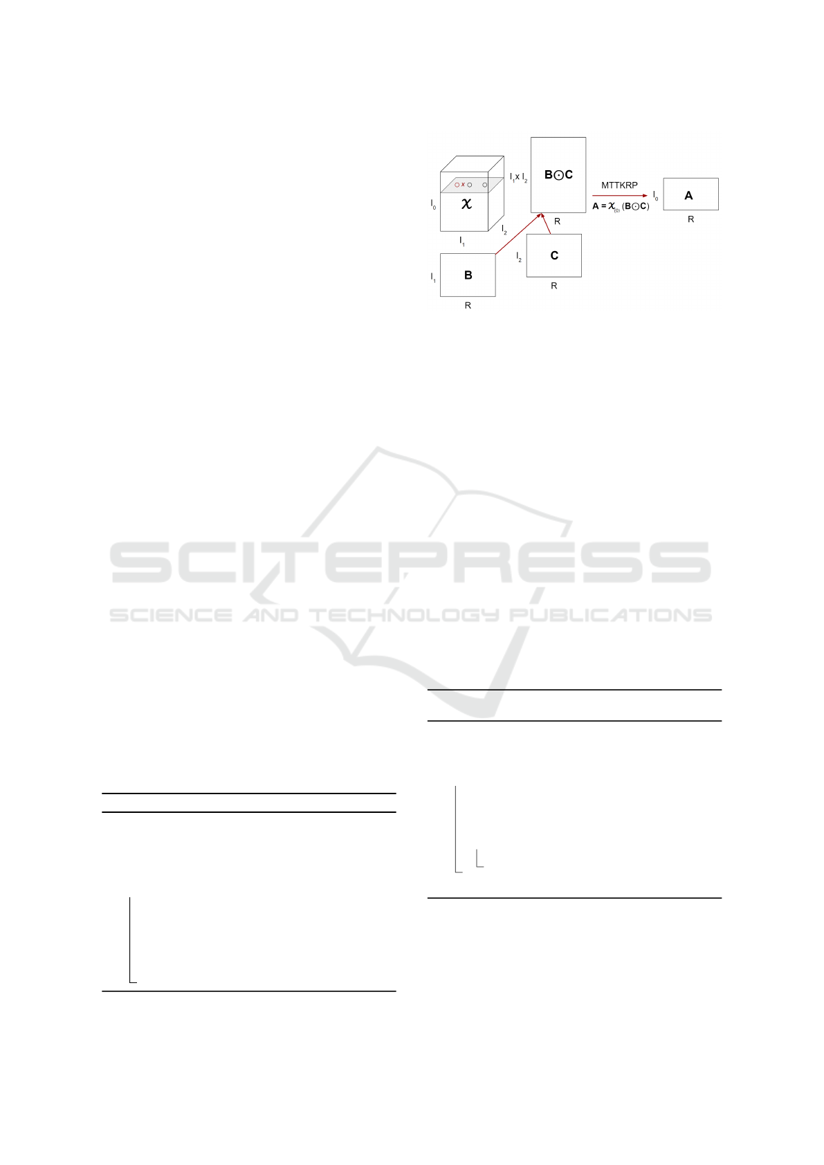
Figure 1: An illustration of MTTKRP for a 3D tensor X in

mode 0.

Figure 1 illustrates the update process of MT-

TKRP for mode 0. With a sparse tensor stored in the

coordinate format, sparse MTTKRP (spMTTKRP)

for mode 0 can be performed as shown in Algo-

rithm 1. For each non-zero element x in a sparse 3D

tensor X ∈ R

×I

at (i, j, k), the ith row of A is up-

dated as follows: the jth row of B and the kth row of C

are fetched, and their Hadamard product is computed

and scaled with the value of x. The main challenge

for efﬁcient computation is how to access the factor

matrices and non-zero elements for the spMTTKRP

operation. We will use a hypergraph model for mod-

eling these dependencies in the spMTTKRP operation

in Section 3.

Algorithm 2 shows the sequential sparse MT-

TKRP (spMTTKRP) approach for third-order tensors

in Coordinate (COO) Format, where IndI, indJ, and

indK correspond to the coordinate vectors of each

non-zero tensor element. “nnz” refers to the number

of non-zero values inside the tensor.

Algorithm 2: Single iteration of COO based spMTTKRP

for third order tensors.

Input: indI[nnz], indJ[nnz], indK[nnz],

vals[nnz], B[J][R], C[K][R]

Output:

A[I][R]

1 for z = 0 to nnz−1 do

2 i = indI[z]

3 j = indJ[z]

4 k = indK[z]

5 for r = 0 to R−1 do

A[i][r] += vals[z] · B[j][r] · C[k][r]

7 return

2.2 FPGA Technologies

FPGAs are especially suitable for accelerating

memory-bound applications with irregular data ac-

cesses which require custom hardware. The logic

Towards Programmable Memory Controller for Tensor Decomposition

469

cells on state-of-the-art FPGA devices consist of

Look Up Tables (LUTs), multiplexers, and ﬂip-ﬂops.

FPGA devices also have access to a large on-chip

memory (BRAM). High-bandwidth interfaces to ex-

ternal memory can be implemented on FPGA. Cur-

rent FPGAs are comprised of multiple Super Logic

Regions (SLRs), where each SLR is connected to a

single or several DRAMs using a memory interface

IP.

HBM technology is used in state-of-the-art FP-

GAs as the high bandwidth interconnections particu-

larly beneﬁt FPGAs (Kuppannagari et al., 2019). The

combination of high bandwidth access to large banks

of memory from logic layers makes 3DIC architec-

tures attractive for new approaches to computing, un-

constrained by the memory wall. Cache Coherent

Interconnect supports shared memory and cache co-

herency between the processor (CPU) and the accel-

erator. Both FPGA and the processor have access to

shared memory in the form of external DRAM, while

the cache coherency protocol ensures that any mod-

iﬁcations to a local copy of the data in either device

are visible to the other device. Protocols such as CXL

(CXL, 2021) and CCIX (CCIX, 2021) develop to re-

alize coherent memory.

3 SPARSE MTTKRP COMPUTE

PATTERNS

The spMTTKRP operation for a given tensor can

be represented using a hypergraph. For illustrative

purposes, we consider a 3 mode sparse tensor X ∈

×I

where (i

, i

) denote the coordinates of x

in X . Here I

, I

, and I

represent the size of each ten-

sor mode. Note that the following approaches can be

applied to tensors with any number of modes.

For a given tensor X , we can build a hypergraph

H = (V, E) with the vertex set V and the hyperedge set

E as follows: vertices correspond to the tensor indices

in all the modes and hyperedges represent its non-zero

elements. For a 3D sparse tensor X ∈ R

×I

with

M non-zero elements, its hypergraph H = (V, E) con-

sists of |V | = I

+ I

vertices and |E| = M hy-

peredges. A hyperedge X (i, j, k) connects the three

vertices i, j, and k, which correspond to the indices of

rows of the factor matrices. Figure 2 shows an exam-

ple of the hypergraph for a sparse tensor.

Our goal is to determine a mapping of X into

memory for each mode so that the total time spent

on (1) loading tensor data from external memory, (2)

loading input factor matrix data from the external

memory, (3) storing output factor matrix data to the

external memory, and (4) element-wise computation

Figure 2: A hypergraph example of a sparse tensor.

for each non-zero element of the tensor is minimized.

Considering the current works in the literature

(Srivastava et al., 2019) (Nisa et al., 2019) (Li et al.,

2018) (Helal et al., 2021), for a given mode, there are

2 ways to perform sparse MTTKRP.

• Approach 1: Output-mode direction computation

• Approach 2: Input-mode direction computation

Algorithm 3 and Algorithm 4 show the mode 0

MTTKRP of a tensor with three modes using Ap-

proach 1 and Approach 2, respectively.

Algorithm 3: Approach 1 for mode 0 of a tensor with 3

modes.

1 Input: A sparse tensor X ∈ R

×I

, dense

factor matrices B ∈ R

×R

, C ∈ R

×R

2 Output: Updated dense factor matrix

A ∈ R

×R

3 for each i

output factor matrix row in A do

4 A(i

, :) = 0

5 for each nonzero element in X at

, i

) with i

coordinates do

6 Load(X (i

, i

))

7 Load(B(i

, :))

8 Load(C(i

, :))

9 for r = 1, . . . , R do

10 A(i

, r)+ =

X (i

, i

) × B(i

, r) × C(i

, r)

11 Store(A(i

, :))

12 return A

We use the hypergraph model of the tensor to

describe the different approaches. The main differ-

ence between these two approaches is the hypergraph

traversal order. Hence, we denote the two approaches

based on the order of hyperedge traversal.

In Approach 1, all hyperedges that share the same

vertex of the output mode are accessed consecutively.

For each hyperedge, all the input vertices are tra-

versed to access their corresponding rows of input

factor matrices. In Approach 2, all hyperedges that

share the same vertex of one of the input modes are

DATA 2022 - 11th International Conference on Data Science, Technology and Applications

470

Algorithm 4: Approach 2 for mode 0 of a tensor with 3

modes.

1 Input: A sparse tensor X ∈ R

×I

, dense

factor matrices B ∈ R

×R

, C ∈ R

×R

2 Output: Updated dense factor matrix

A ∈ R

×R

3 for each i

input factor matrix row in B do

4 Load(B(i

, :))

5 for each nonzero element in X at

, i

) with i

coordinates do

6 Load(X (i

, i

))

7 Load(C(i

, :))

8 for r = 1, . . . , R do

9 p

, r) =

X (i

, i

) × B(i

, r) × C(i

, r)

10 Store(p

, :))

11 for each i

output factor matrix row in A

12 A(i

, :) = 0

13 for each partial element p

with i

coordinates do

14 for r = 1, . . . , R do

15 Load(p

, :))

16 A(i

, r)+ = p

, r)

17 Store(A(i

, :))

18 return A

19 SetAlFnt

accessed sequentially. For each vertex, all its incident

hyperedges are iterated consecutively. For each hy-

peredge, the rest of the input vertices of the hyperedge

are traversed to access rows of the remaining input

factor matrices. It follows the element-wise multipli-

cation and addition.

In Approach 1, since the order of hyperedge de-

pends on the output mode, the output factor ma-

trix can be calculated without generating intermediate

partial sums (Algorithm 3: line 10). However, in Ap-

proach 2, since the hyperedges are ordered according

to the input mode coordinates, we need to store the

partial sums (Algorithm 4: line 9) in the FPGA exter-

nal memory. It leads to accumulating the partial sums

to generate the output factor matrix (Algorithm 4: line

11-17).

The total computations of both approaches are

the same: for a general sparse tensor with |T | non-

zero elements, N modes, and factor matrices with

rank R, since every hyperedge will be traversed once,

and there are N − 1 multiplications and one addition

for computing MTTKRP, the total computation per

mode is N × |T | × R. However, their total external

memory accesses are different: both approaches re-

quire |T | load operations for all the hyperedges and

the total factor matrix elements transferred per mode

is (N − 1) × |T | × R, which corresponds to access-

ing input factor matrices of vertices in the hyper-

graph model. However, in Approach 2, the partial

value needs to be stored in the memory (Algorithm 4:

line 10), which requires an additional |T | × R exter-

nal memory storage. Let I

out

and I

represent the

length of the output mode and the input mode, respec-

tively. Then the total amount of data transferred is

|T | + (N − 1) × |T | ×R + I

out

× R for Approach 1 and

|T | +N ×|T |×R + I

×R for Approach 2. Therefore,

Approach 1 beneﬁts from avoiding loading and stor-

ing partial sums. Table 1 summarizes the properties

of the two approaches.

Table 1: Comparison of the Approaches.

Approach Total Computations Total external memory accesses Size of total partial sums

1 N × |T | × R |T | + (N −1) × |T | × R + I

out

× R 0

2 N × |T | × R |T | + N ×|T | × R +I

× R |T | × R

In the following, we discuss these in detail and

identify the memory access characteristics.

3.1 spMTTKRP on FPGA

In this paper, we consider large-scale data decompo-

sition on very large tensors. Hence the FPGA stores

the tensor and the factor matrices inside their exter-

nal DRAM memory. Therefore, we need to optimize

the FPGA memory controller to the DRAM technol-

ogy. In this section, we ﬁrst explain the DRAM tim-

ing model following the memory access patterns of

sparse MTTKRP. Figure 3 shows the conceptual over-

all design.

Approach 2 is not practical for FPGA due to the

large external memory requirement to store the par-

tial sums during the computation. In the work of this

paper, we focus on Approach 1.

For Approach 1, the tensor is sorted according to

the coordinates of the output mode. Typically, spMT-

TKRP is calculated for all the modes. To adapt Ap-

proach 1 to compute the factor matrices correspond-

ing to all the modes, (1) Use multiple copies of the

tensor. Each tensor copy is sorted according to the co-

ordinates of a tensor mode or (2) re-order the tensor

in the output direction before computing spMTTKRP

for a mode.

Using multiple copies of a tensor is not a prac-

tical solution due to the limited external memory of

the FPGA. Hence, our memory solution focuses on

remapping the tensor in the output direction before

computing spMTTKRP for a mode. It enables to per-

form spMTTKRP using Approach 1 for each tensor

mode.

Towards Programmable Memory Controller for Tensor Decomposition

471

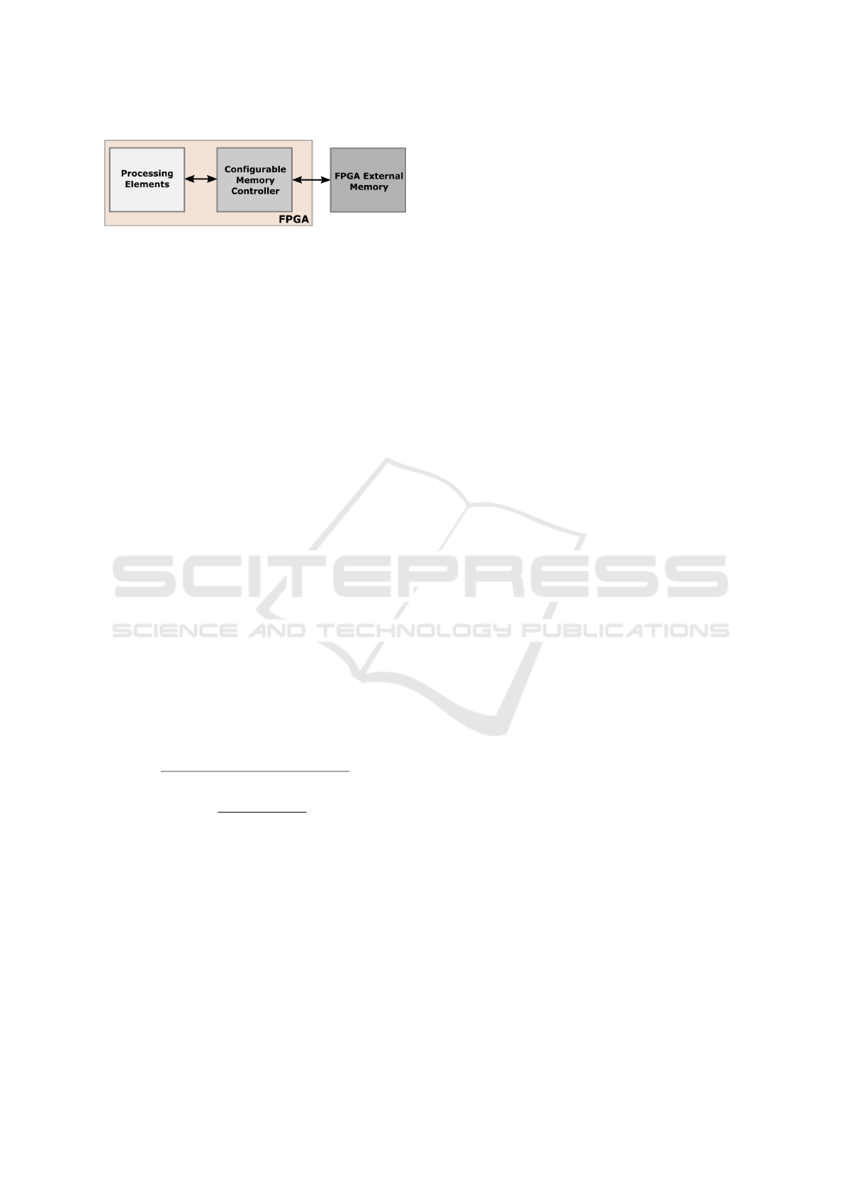
Figure 3: Conceptual overall design.

Algorithm 5 summarizes the Approach 1 with

remapping. The algorithm focus on computing spMT-

TKRP of mode 1. Initially, we assume the sparse ten-

sor is ordered according to the coordinates of mode

0 after computing the factor matrix of mode 0. Be-

fore starting the spMTTKRP for mode 1, we remap

the according to the mode 1 coordinates (lines 3 -

6). After remapping, all the non-zero values with

the same output mode coordinates are brought to the

compute unit consecutively (line 9). For each non-

zero value, the corresponding rows of the input factor

matrices are brought into the compute units following

the element-wise multiplication and addition. Since

the tensor elements with the same output mode coor-

dinates are brought together, the processing unit can

calculate the output factor matrix without storing the

partial values in FPGA external memory. Once a row

of factor matrix is computed, the value is stored in

the external memory. Here, Load/Store corresponds

to loading/storing an element from the external mem-

ory. Also, “:” refers to performing an operation for an

entire factor matrix row.

The proposed approach introduces several imple-

mentation overheads:

Additional External Memory Accesses:

The remapping required additional external memory

load and a store (Algorithm 5: lines 4 and 6). The

total access to the external memory is increased by

2 × |T | for a tensor of size |T |. The communication

overhead per mode is:

2 × |T |

|T | + (N − 1) × |T | × R + I

out

× R

≈

1 + (N − 1) × R

For a typical scenario (N = 3-5 and R = 16-64), the

total external memory communication only increases

by less than 6%.

Additional External Memory Space:

During the remapping process, the remapped data re-

quires an additional space equal to the size of the ten-

sor (|T |) to store the remapped tensor elements in the

memory.

Excessive Memory Address Pointers to Store the

Remapped Tensor:

The remapping brings the tensor elements with the

same output mode coordinate together (Algorithm 5:

line 5). To achieve this, the memory controller needs

to track the memory location (i.e., memory address)

of the next tensor element with each output coordinate

needs to be stored. This required memory address

pointers, which track the memory address to store a

tensor element depending on its output mode coor-

dinate. Algorithm 5 requires such memory pointers

proportionate to the size of the output mode of a given

tensor.

The number of address pointers may not ﬁt in the

FPGA internal memory for a large tensor. For ex-

ample, a tensor with an output mode with 10 million

coordinate values requires 40 MB to store the mem-

ory address pointers (i.e., 32-bit memory addresses

are considered). It does not ﬁt in the FPGA on-chip

memory. Hence the address pointers should be stored

in the external memory. It introduces additional ex-

ternal memory access for each tensor element.

Also, the number of tensor elements with the same

output mode coordinate value is different for each

output coordinate due to the sparsity of the tensor. It

complicates the memory layout of the tensor.

An ideal memory layout should guarantee: (1)

The number of memory address pointers required for

remapping ﬁt in the internal memory of the FPGA,

and (2) Each tensor partition contains the same num-

ber of tensor elements.

4 SPARSE MTTKRP MEMORY

ACCESS PATTERNS

The proposed sparse MTTKRP computation has 5

main actions: (1) load a non-zero tensor element,

(2) load corresponding factor matrices, (3) perform

spMTTKRP operation, (4) store remapped tensor el-

ements, and (5) store the ﬁnal output.

The objective of the memory controller is to de-

crease the total DRAM memory access time. To iden-

tify the opportunities to reduce the memory access

time, we analyze the memory access patterns of the

proposed tensor format and memory layout. The sum-

mary of memory access patterns is as follows:

1. The tensor elements can be loaded as streaming

accesses while remapping and computing spMT-

TKRP.

2. Each remapped tensor element can be stored

element-wise.

3. The different rows of each input factor matrices

are random accesses.

4. Each rows of output factor matrix can be stored in

streaming memory access.

DATA 2022 - 11th International Conference on Data Science, Technology and Applications

472

Algorithm 5: Approach 1 with remapping for mode 1 of a

tensor with 3 modes.

1 Input: A sparse tensor X ∈ R

×I

sorted in

mode 0, dense factor matrices A ∈ R

×R

C ∈ R

×R

2 Output: Updated dense factor matrix

B ∈ R

×R

3 for each non-zero element in X at (i

, i

)

with i

coordinates do

4 Load(X (i

, i

))

5 pos

= Find(Memory address of i

)

6 Store(X (i

, i

) at memory address

pos

)

7 for each i

output factor matrix row in B do

8 B(i

, :) = 0

9 for each non-zero element in X at

, i

) with i

coordinates do

10 Load(X (i

, i

))

11 Load(A(i

, :))

12 Load(C(i

, :))

13 for r = 1, . . . , R do

14 B(i

, r)+ =

X (i

, i

) × A(i

, r) × C(i

, r)

15 Store(B(i

, :))

16 return B

Accessing the data in bulk (i.e., a large chunk of

data stored sequentially) can reduce the total mem-

ory access time. It is due to the characteristics of

the DRAM. DMA (Direct Memory Access) is the

standard method to perform bulk memory transfers.

Further, the random accesses can be performed as

element-wise memory accesses through a cache to ex-

plore the temporal and spatial locality of the accesses.

It can improve the total access time.

Thus memory transfer types are as follows:

1. Cache Transfers: Supports random memory ac-

cesses. Load/store individual requests in mini-

mum latency. Access patterns with high spatial

and temporal locality are transferred using cache

lines.

2. DMA Stream Transfers: Supports streaming ac-

cesses. Load/store operations on all requested

data with minimum latency from memory.

3. DMA Element-wise Transfers: Transfer the re-

quested data element-wise. This method is used

with data with no spatial and temporal locality.

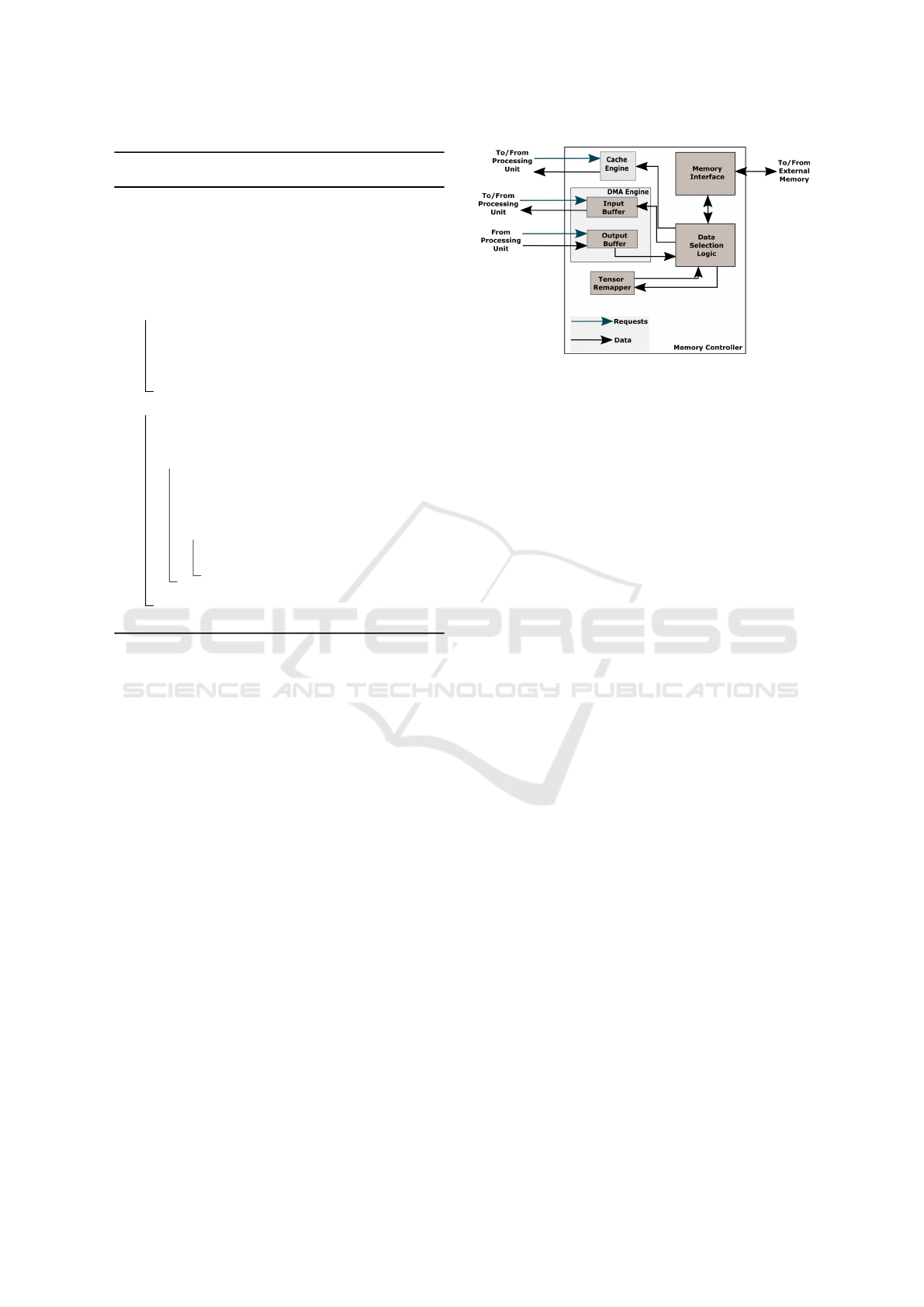
Figure 4: Proposed Memory Controller.

5 TOWARDS CONFIGURABLE

MEMORY CONTROLLER

To support the memory accesses, we propose a pro-

grammable memory controller as shown in Figure 4.

It consists of a Cache Engine, a tensor remapper, and a

DMA Engine. We evaluate the impact of using caches

and DMAs as intermediate buffering techniques to re-

duce the total execution time of sparse MTTKRP.

The modules inside the memory controller (e.g.,

Cache Engine, tensor remapper, and DMA Engine)

can be developed as conﬁgurable hardware. These

modules are programmable during the FPGA synthe-

sis time. For example, the Cache Engine can have a

different number of cache lines and associativity that

can be conﬁgured during synthesis time. Also, the

resource utilization of each module heavily depends

on the conﬁguration. On the other hand, the FPGA

contains limited on-chip resources. Hence the FPGA

resources should be distributed among different mod-

ules optimally, such that the overall memory access

time is minimized (see Section 5.3).

5.1 Memory Controller Architecture

5.1.1 Cache Engine

The Cache Engine can be used to satisfy a single

memory request with minimum latency. The Cache

Engine is used to explore the spatial and temporal lo-

cality of requested data. We intend to use Cache En-

gine to explore the locality of the input factor matri-

ces. When a tensor computation requests a row of the

factor matrix, the memory controller ﬁrst look-ups the

Cache Engine. If the requested factor matrix row is al-

ready in the Cache Engine due to prior requests, the

factor matrix row is forwarded to the tensor compu-

tation from the Cache Engine. Otherwise, the tensor

row is loaded to the Cache Engine from the FPGA

external memory. Then a copy of the matrix row is

Towards Programmable Memory Controller for Tensor Decomposition

473

forwarded to the computation while storing it in the

cache.

5.1.2 DMA Engine

The DMA Engine can process bulk transfers between

the compute units inside FPGA and FPGA external

memory. A DMA Engine can have several DMA

buffers inside.

The main advantages of having a DMA Engine

are: (a) DMA requests can request more than one el-

ement at once, unlike the Cache Engine, and reduce

the input trafﬁc of the memory controller, (b) Using

a DMA Engine to access data without polluting the

cache inside the Cache Engine, and (c) DMA trans-

fers can utilize the external memory bandwidth for

bulk transfers.

5.1.3 Tensor Remapper

Tensor remapper includes a DMA buffer and the

proposed remapping logic discussed in Section

3. It loads each partition of the tensor as a bulk

transfer similar to the DMA Engine. After, it stores

each tensor element depending on the output mode

coordinate value in an element-wise fashion.

Required Memory Consistency of the Mem-

ory Controller:

The suggested memory controller above should have

a weak memory consistency model with the following

properties:

• Consistency of DMA Engine, Cache Engine

and Tensor Remapper: They processes its re-

quests based on a ﬁrst-in-ﬁrst-out basis.

• Consistency between Cache Engine, Tensor

Remapper and DMA Engine: The ﬁrst-in ﬁrst-

served basis is maintained. Since the same mem-

ory location is not accessed by the Cache Engine,

Tensor Remapper and DMA Engine at the same

time, weak consistency is maintained.

5.2 Programmable Parameters

The Cache Engine and DMA Engine use on-chip

FPGA memory (i.e., BRAM and URAM). These re-

sources need to be shared among the modules opti-

mally to achieve signiﬁcant improvements in memory

access time. The resource requirement of the Cache

Engine and DMA Engine depends on their conﬁg-

urable parameters mentioned below.

Table 2: Characteristics of sparse tensors in FROSTT

Repository.

Metric Value

Length of a tensor mode 17-39 M

Width of a matrix (R) 8 − 32 (Typical = 16)

Number of non-zeros 3-144 M

Number of modes 3, 4, 5

Tensor size ≤ 2.25 GB

Size of a factor matrix < 4.9 GB

5.2.1 Memory Controller Parameters

Cache Engine parameters include cache line width,

number of cache lines, and associativity of the cache.

The design parameters of the DMA Engine are:

the number of DMAs, the number of DMA buffers

per DMA, and the size of DMA buffers.

The design parameters of the Tensor Remapper in-

clude: (1) size of the DMA buffer, (2) width of a ten-

sor element, and (3) the maximum number of address

pointers Tensor Remapper can track.

5.3 Exploring the Design Space

The tensor datasets can have different characteristics

depending on the domain from which the dataset is

extracted. Table 2 shows the characteristics of the

tensors in The Formidable Repository of Open Sparse

Tensors and Tools (FROSTT) (Smith et al., 2017). It

is commonly used in the high-performance comput-

ing community to benchmark custom accelerator de-

signs for sparse MTTKRP.

Tensor datasets from separate domains of appli-

cations have different characteristics such as sparsity,

size of the modes, and the number of modes. Hence,

the datasets extracted from various applications show

the least memory access time with different conﬁg-

urations of the memory controller. Hence, perfor-

mance estimator software is required to estimate the

optimal conﬁgurable parameters for datasets of a do-

main. We introduce the features of a Performance

Model Simulator (PMS) software to estimate the to-

tal execution time of spMTTKRP for a given dataset.

It can use with multiple datasets from the same do-

main to estimate the average execution time (t

avg

) for

a selected domain. Also, it should estimate the total

FPGA on-chip memory requirement for a given set

of programmable parameters to make sure the mem-

ory controller ﬁts in the FPGA device. We will ex-

plore the possible inputs required for a PMS concern-

ing: (1) available FPGA resources (i.e., total BRAMs,

and URAMs of the selected FPGA and data width of

memory interface), (2) size of data structures (e.g.,

size of an input tensor element, size of an input fac-

DATA 2022 - 11th International Conference on Data Science, Technology and Applications

474

tor matrix element, and rank of the input factor ma-

trices), and (3) Parameters of the memory controller

(i.e., DMA buffer sizes, number of cache lines, as-

sociativity of cache, and number of factor matrices

shared by a cache).

A module-by-module (e.g., Cache Engine and

DMA Engine) exhaustive parameter search can be

proposed to identify the optimal parameters for the

memory controller.

6 DISCUSSION

In this paper, we investigated the characteristics of a

custom memory controller that can reduce the total

memory access time of sparse MTTKRP on FPGAs.

Sparse MTTKRP is a memory-bound operation. It

has 2 types of memory access patterns that can be op-

timized to reduce the total memory access time. A

memory controller design that can be conﬁgured dur-

ing compile/synthesis time depending on the applica-

tion and targeted hardware is required.

We are developing a conﬁgurable memory con-

troller and a memory layout for sparse tensors to re-

duce the total memory access time of sparse MT-

TKRP operation.

Since synthesizing a FPGA can take a long time,

optimizing the memory controller parameters for a

given application can be a time-consuming process.

Hence, we are developing a Performance Model Sim-

ulator (PMS) software to identify the optimal param-

eters for a given application on a selected FPGA.

ACKNOWLEDGEMENTS

This work was supported by the U.S. National Sci-

ence Foundation (NSF) under grants NSF SaTC #

2104264 and PPoSS- 2119816.

REFERENCES

CCIX (2021). Cache Coherent Interconnect for Accelera-

tors (CCIX). https://www.ccixconsortium.com/.

Cheng, Z., Li, B., Fan, Y., and Bao, Y. (2020). A novel

rank selection scheme in tensor ring decomposition

based on reinforcement learning for deep neural net-

works. In ICASSP 2020-2020 IEEE International

Conference on Acoustics, Speech and Signal Process-

ing (ICASSP), pages 3292–3296. IEEE.

CXL (2021). Compute Express Link (CXL).

https://www.computeexpresslink.org/.

Helal, A. E., Laukemann, J., Checconi, F., Tithi, J. J.,

Ranadive, T., Petrini, F., and Choi, J. (2021). Alto:

Adaptive linearized storage of sparse tensors. In Pro-

ceedings of the ACM International Conference on Su-

percomputing, ICS ’21, page 404–416, New York,

NY, USA. Association for Computing Machinery.

Kolda, T. G. and Bader, B. W. (2009). Tensor decomposi-

tions and applications. SIAM review, 51(3):455–500.

Kuppannagari, S. R., Rajat, R., Kannan, R., Dasu, A., and

Prasanna, V. (2019). Ip cores for graph kernels on fp-

gas. In 2019 IEEE High Performance Extreme Com-

puting Conference (HPEC), pages 1–7.

Li, J., Sun, J., and Vuduc, R. (2018). Hicoo: Hierarchical

storage of sparse tensors. In Proceedings of the Inter-

national Conference for High Performance Comput-

ing, Networking, Storage, and Analysis, SC ’18. IEEE

Press.

Mondelli, M. and Montanari, A. (2019). On the connec-

tion between learning two-layer neural networks and

tensor decomposition. In The 22nd International Con-

ference on Artiﬁcial Intelligence and Statistics, pages

1051–1060. PMLR.

Nisa, I., Li, J., Sukumaran-Rajam, A., Vuduc, R., and Sa-

dayappan, P. (2019). Load-balanced sparse mttkrp on

gpus. In 2019 IEEE International Parallel and Dis-

tributed Processing Symposium (IPDPS), pages 123–

133.

Smith, S., Choi, J. W., Li, J., Vuduc, R., Park, J., Liu, X.,

and Karypis, G. (2017). FROSTT: The formidable

repository of open sparse tensors and tools.

Srivastava, N., Rong, H., Barua, P., Feng, G., Cao,

H., Zhang, Z., Albonesi, D., Sarkar, V., Chen,

W., Petersen, P., Lowney, G., Herr, A., Hughes,

C., Mattson, T., and Dubey, P. (2019). T2s-

tensor: Productively generating high-performance

spatial hardware for dense tensor computations. In

2019 IEEE 27th Annual International Symposium on

Field-Programmable Custom Computing Machines

(FCCM), pages 181–189.

Wen, F., So, H. C., and Wymeersch, H. (2020). Ten-

sor decomposition-based beamspace esprit algorithm

for multidimensional harmonic retrieval. In ICASSP

2020-2020 IEEE International Conference on Acous-

tics, Speech and Signal Processing (ICASSP), pages

4572–4576. IEEE.

Xilinx (2019). Alveo u250 data center accelerator

card. https://www.xilinx.com/products/boards-and-

kits/alveo/u250.html.

Towards Programmable Memory Controller for Tensor Decomposition

475